Chapter 14 Alternative-Specific Multinomial Logit Models

14.1 Introduction: Why Alternative-Specific MNL?

In the last chapter, we modeled brand choice using standard multinomial logit (MNL) models, where all predictors were case-specific. That is, they described the consumer or choice situation and took the same value for all brands in a given choice set.

In many real marketing applications, however, the most important predictors vary by brand. Examples include:

• Price of each brand
• Package size
• Sugar content or nutritional attributes
• Promotional indicators
• Brand-specific features

Alternative-specific multinomial logit (AS-MNL) models allow us to include these variables directly, providing richer managerial insight into how brand attributes drive choice.

In this chapter, you will learn how to:

• Work with long-format choice data
• Split alternative-specific data correctly into training and test samples
• Estimate an alternative-specific MNL model
• Evaluate model fit and classification performance
• Interpret predicted probabilities and marginal effects in a marketing context

Throughout the chapter, we will use the yogurt dataset.

---

14.2 The Yogurt Choice Data

The yogurt dataset records consumer brand choices in repeated choice situations. Each row represents one alternative within one choice situation, not a single consumer.

Key implications:

• Each choice situation appears multiple times (once per brand)
• Exactly one alternative is chosen per choice set
• Many predictors vary across brands within the same choice set

This “long” structure is required for alternative-specific MNL models and differs from the wide-format data used earlier in the course.

---

14.3 Preparing the Data for Modeling

14.3.1 Why Splitting Is Different for Choice Data

With alternative-specific data, we cannot randomly split rows into training and test sets. Doing so would break apart choice sets and contaminate model evaluation.

Instead, we must split at the choice-set level, ensuring that all rows belonging to the same choice situation stay together.

14.3.2 Creating Training and Test Samples

We still use the splitsample() function from the MKT4320BGSU package, which supports group-level splitting. Whereas before we didn’t use several parameters, will will use them for alternative specific MNL.

Usage:

• splitsample(data, outcome = NULL, group = NULL, choice = NULL, alt = NULL,
p = 0.75, seed = 4320)
• where:
  • data is the data frame to split, in long-format.
  • outcome is NOT (USUALLY) USED FOR ALTERNATIVE SPECIFIC MNL
  • group is the grouping variable (e.g., choice situation id or respondent id). If provided, splitting is done at the group level. Required for alternative specific MNL.
  • choice is the 0/1 (or TRUE/FALSE) indicator for the chosen alternative. Used only when group is provided. Required for alternative specific MNL.
  • alt is the optional alternative label/ID. Used with choice to stratify at the group level. Required for alternative specific MNL.
  • p is the proportion of observations to place in the training set. Must be strictly between 0 and 1. Default is 0.75.
  • seed is the random seed for reproducibility. Default is 4320.

Before, we were interested in the $train and $test data frames. Now, we are interested in the train.mdata and test.mdata objects that are saved. They are in the format needed for the using mlogit (see below). However, to avoid a console error, you’ll access the a slightly different way.

sp <- splitsample(data = yogurt, group = "id", choice = "choice", alt = "brand")

train <- sp[["train.mdata"]]
test  <- sp[["test.mdata"]]

At this point:

• train contains complete choice sets for model estimation
• test contains unseen choice sets for out-of-sample evaluation

---

14.4 Specifying an Alternative-Specific MNL Model

In an alternative-specific MNL model:

• Case-specific variables enter once
• Alternative-specific variables enter as brand-varying predictors

We use the mlogit function from the mlogit package to estimate the model. We separate the alternative specific from the case specific variables with a |. Alternative specific come first, then the case specific. We can use the base R summary() function to get the raw log-odds estimates.

library(mlogit)
as_mnl_fit <- mlogit(choice ~ price + feat | income, data = train)
summary(as_mnl_fit)

Call:
mlogit(formula = choice ~ price + feat | income, data = train, 
    method = "nr")

Frequencies of alternatives:choice
  Dannon   Hiland   Weight  Yoplait 
0.401988 0.029818 0.229155 0.339039 

nr method
8 iterations, 0h:0m:0s 
g'(-H)^-1g = 0.000171 
successive function values within tolerance limits 

Coefficients :
                      Estimate Std. Error  z-value  Pr(>|z|)    
(Intercept):Hiland   0.7587200  0.5677111   1.3365  0.181401    
(Intercept):Weight  -0.0263906  0.2078931  -0.1269  0.898986    
(Intercept):Yoplait -3.9886941  0.2679762 -14.8845 < 2.2e-16 ***
price               -0.4424450  0.0295572 -14.9691 < 2.2e-16 ***
feat                 0.4230830  0.1491240   2.8371  0.004552 ** 
income:Hiland       -0.1081164  0.0149201  -7.2464 4.281e-13 ***
income:Weight       -0.0114764  0.0037707  -3.0436  0.002338 ** 
income:Yoplait       0.0729207  0.0040281  18.1030 < 2.2e-16 ***
---
Signif. codes:  0 '***' 0.001 '**' 0.01 '*' 0.05 '.' 0.1 ' ' 1

Log-Likelihood: -1618.4
McFadden R^2:  0.23972 
Likelihood ratio test : chisq = 1020.6 (p.value = < 2.22e-16)

Interpretation notes:

• Coefficients reflect changes in relative utility
• Signs and magnitudes should be interpreted in marketing terms
• Alternative-specific variables capture within-choice substitution effects

---

14.5 Evaluating Model Performance

14.5.1 Model Fit and Coefficients

We use the eval_as_mnl() function from the MKT4320BGSU package to obtain fit statistics, coefficients (both log-odds and odds ratio), and classification diagnostics.

Usage:

• eval_as_mnl(model, digits = 4, ft = FALSE, newdata = NULL,
label_model = "Model data", label_newdata = "New data", class_digits = 3)
• where:
  • model is a fitted mlogit model.
  • digits is an integer; decimals to round coefficient and fit results (default 4).
  • ft is logical; if TRUE, return coefficient and classification tables as flextable objects (default FALSE).
  • newdata is an optional dfidx object (e.g., test.mdata) for an additional classification matrix. If NULL, only the training-data matrix is produced.
  • label_model is a character string label for the training-data classification matrix (default “Model data”).
  • label_newdata is a character string label for the newdata classification matrix (default “New data”).
  • class_digits is an integer; decimals to round classification results (default 3).

Key outputs include:

• Log-likelihood \(\chi^2\) test
• McFadden’s pseudo \(R^2\)
• Odds ratios for interpretation
• Classification accuracy and diagnostics

as_eval <- eval_as_mnl(as_mnl_fit, ft = TRUE, newdata = test)
as_eval$coef_table

LR chi2 (5) = 1020.5649; p < 0.0001
McFadden's Pseudo R-square = 0.2397
term	logodds	OR	std.error	statistic	p.value
(Intercept):Hiland	0.7587	2.1355	0.5677	1.3365	0.1814
(Intercept):Weight	-0.0264	0.9740	0.2079	-0.1269	0.8990
(Intercept):Yoplait	-3.9887	0.0185	0.2680	-14.8845	0.0000
price	-0.4424	0.6425	0.0296	-14.9691	0.0000
feat	0.4231	1.5267	0.1491	2.8371	0.0046
income:Hiland	-0.1081	0.8975	0.0149	-7.2464	0.0000
income:Weight	-0.0115	0.9886	0.0038	-3.0436	0.0023
income:Yoplait	0.0729	1.0756	0.0040	18.1030	0.0000

as_eval$classify_model

Classification Matrix - Model data
Accuracy = 0.621
PCC = 0.330
	Reference
Predicted	Dannon	Hiland	Weight	Yoplait	Total
Dannon	577	39	324	97	1037
Hiland	1	12	0	2	15
Weight	18	2	38	18	76
Yoplait	132	1	53	497	683
Total	728	54	415	614	1811
Statistics by Class:
Sensitivity	0.793	0.222	0.092	0.809
Specificity	0.575	0.998	0.973	0.845
Precision	0.556	0.800	0.500	0.728

as_eval$classify_newdata

Classification Matrix - New data
Accuracy = 0.607
PCC = 0.331
	Reference
Predicted	Dannon	Hiland	Weight	Yoplait	Total
Dannon	199	14	104	38	355
Hiland	2	2	1	1	6
Weight	8	1	12	13	34
Yoplait	33	0	21	152	206
Total	242	17	138	204	601
Statistics by Class:
Sensitivity	0.822	0.118	0.087	0.745
Specificity	0.565	0.993	0.952	0.864
Precision	0.561	0.333	0.353	0.738

14.5.2 Classification Performance

Classification is evaluated at the choice-set level:

• The predicted brand is the one with the highest predicted probability
• Accuracy reflects correct brand predictions
• PCC provides a baseline comparison

This approach mirrors how managers think about predicting actual consumer choices.

---

14.6 Predicted Probabilities and Marginal Effects

14.6.1 Why Predicted Probabilities Matter

Coefficients are not always intuitive. Predicted probabilities translate the model into outcomes managers care about:

• Market shares
• Brand switching
• Competitive responses

14.6.2 Why Marginal Effects Are Useful

Marginal effects quantify how much choice probabilities change in response to a small change in an attribute, holding everything else constant. Marginal effects can be computed in two common ways:

• At observed values (Average Marginal Effects, AME)
  Marginal effects are calculated for each observation using its actual attribute values and then averaged.
• At means (Marginal Effects at the Mean, MEM)
  Marginal effects are calculated at a single “average” profile, where each attribute is set to its sample mean.

Both approaches summarize how sensitive choice probabilities are to changes in attributes, but they differ in interpretation.

Marginal effects at observed values:

• Reflect the full distribution of the data
• Avoid relying on a potentially unrealistic “average consumer”
• Are often preferred for descriptive and policy interpretation

Marginal effects at means:

• Are easier to reproduce by hand or with software defaults
• Provide a clear, single reference point
• Can be useful for illustrating model mechanics and comparing effects across variables

The marginal effects tables can therefore answer questions such as:

• “On average, how does a $1 increase in price affect brand choice?”
• “How would choice probabilities change for a typical consumer if an attribute increased slightly?”
• “Which brands are most sensitive to changes in a specific attribute?”

In practice, the choice between observed values and means depends on the goal of the analysis. For interpretation and real-world impact, average marginal effects at observed values are often preferred. For teaching, demonstration, or simplified comparisons, marginal effects at means can be equally informative.

14.6.3 The pp_as_mnl() Function

For both case-specific and alternative-specific predictors, we use the pp_as_mnl() function from the MKT4320BGSU package to get both predicted probabilities and marginal effects.

Usage:

• pp_as_mnl(model,focal_var, focal_type = c("auto", "alt", "case"),
grid_n = 25, digits = 4, ft = FALSE, marginal = TRUE,
me_method = c("observed", "means"), me_step = 1)
• where:
  • model is a fitted mlogit model.
  • focal_var is a character string name of the focal variable.
  • focal_type is a character string; one of “case”, “alt”, or “auto” (default = “auto”).
  • grid_n is an integer; number of points used to construct the grid of focal values for predicted probability plots when the focal variable is continuous (default = 25).
  • digits is an integer; rounding for numeric output (default = 4).
  • ft is logical; if TRUE, return tables as flextable objects (default = FALSE).
  • marginal is logical; if TRUE, compute marginal effects (default = TRUE).
  • me_method is a character string; one of “observed” AME or “means” (default = “observed”).
  • me_step is numeric; finite-difference step size for AME (default = 1).

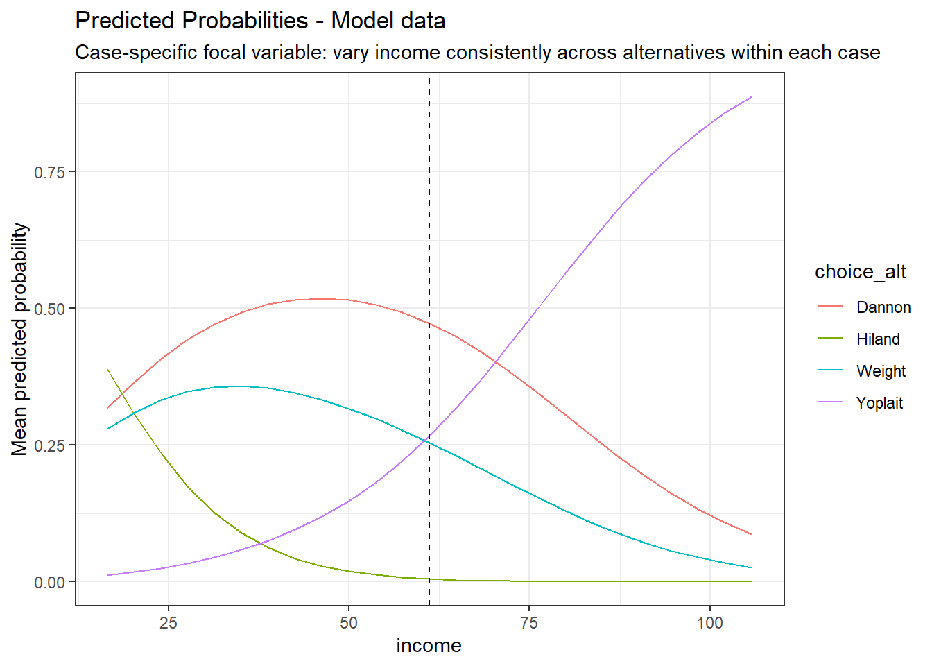
14.6.4 Case-Specific Predictors

We first examine how a consumer-level variable affects brand choice probabilities.

pp_income <- pp_as_mnl(as_mnl_fit, focal_var = "income", ft = TRUE, me_method="means")
pp_income$me_table

Marginal effects for income (at means)
Dannon	Hiland	Weight	Yoplait
-0.0073	-0.0006	-0.0068	0.0147

pp_income$pp_table

Predicted Probability Table (income) - Model data
focal_value	Dannon	Hiland	Weight	Yoplait
60.1438	0.4788	0.0060	0.2608	0.2544
61.1438	0.4729	0.0053	0.2545	0.2672
62.1438	0.4667	0.0047	0.2482	0.2804
Because income is continuous, the values shown include the mean and +/- 1 unit.

pp_income$pp_plot

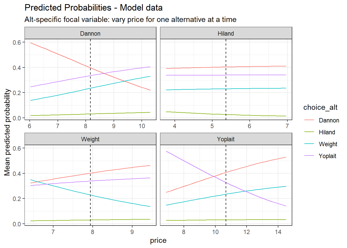
14.6.5 Alternative-Specific Predictors

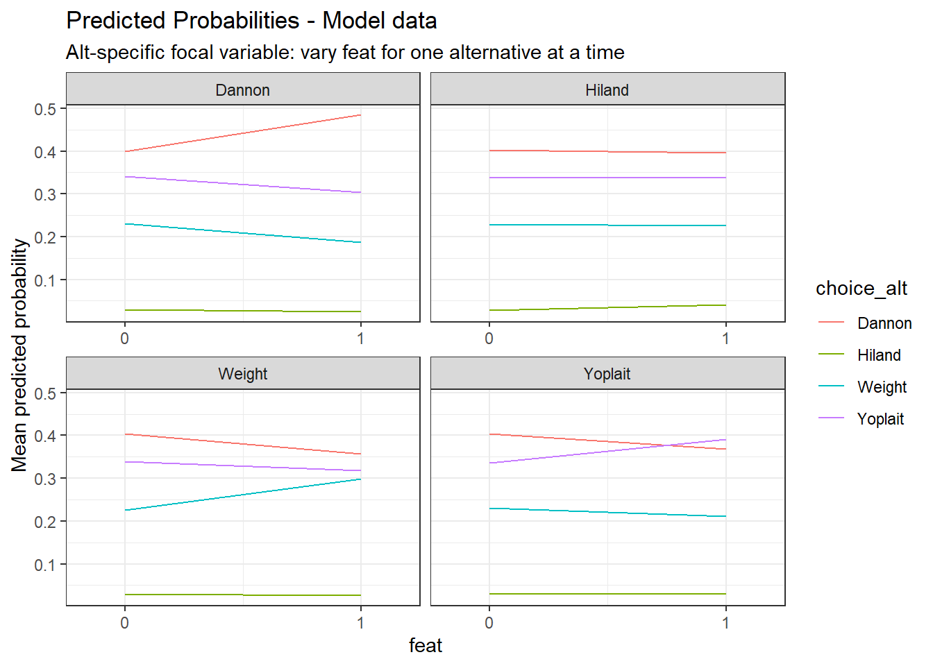
Now we examine a brand-specific variable such as price (a continuous variable) and feature (a categorical variable).

pp_price <- pp_as_mnl(as_mnl_fit, focal_var = "price", ft=TRUE, me_method="means")
pp_price$me_table

Marginal effects for price (at means)
Alternative	Dannon	Hiland	Weight	Yoplait
Dannon	-0.1105	0.0010	0.0550	0.0545
Hiland	0.0010	-0.0021	0.0005	0.0005
Weight	0.0550	0.0005	-0.0845	0.0290
Yoplait	0.0545	0.0005	0.0290	-0.0840

pp_price$pp_table

Predicted Probability Table (price) - Model data
varied_alt	focal_value	Dannon	Hiland	Weight	Yoplait
Dannon	7.1628	0.4918	0.0250	0.1883	0.2949
Dannon	8.1628	0.3980	0.0313	0.2353	0.3355
Dannon	9.1628	0.3088	0.0375	0.2821	0.3716
Hiland	4.3663	0.3966	0.0394	0.2258	0.3382
Hiland	5.3663	0.4035	0.0268	0.2305	0.3392
Hiland	6.3663	0.4083	0.0179	0.2338	0.3399
Weight	6.9421	0.3516	0.0256	0.3060	0.3169
Weight	7.9421	0.4019	0.0301	0.2287	0.3392
Weight	8.9421	0.4446	0.0340	0.1648	0.3566
Yoplait	9.6874	0.3673	0.0302	0.2138	0.3886
Yoplait	10.6874	0.4069	0.0311	0.2350	0.3269
Yoplait	11.6874	0.4438	0.0318	0.2545	0.2699
Because price is continuous, the values shown include the mean and +/- 1 unit.

pp_price$pp_plot

pp_feat <- pp_as_mnl(as_mnl_fit, focal_var = "feat", ft=TRUE, me_method="means")
pp_feat$me_table

Marginal effects for feat (at means)
Alternative	Dannon	Hiland	Weight	Yoplait
Dannon	0.1057	-0.0010	-0.0526	-0.0521
Hiland	-0.0010	0.0020	-0.0005	-0.0005
Weight	-0.0526	-0.0005	0.0808	-0.0277
Yoplait	-0.0521	-0.0005	-0.0277	0.0804

pp_feat$pp_table

Predicted Probability Table (feat) - Model data
varied_alt	focal_value	Dannon	Hiland	Weight	Yoplait
Dannon	0	0.3988	0.0301	0.2308	0.3403
Dannon	1	0.4853	0.0244	0.1870	0.3033
Hiland	0	0.4027	0.0285	0.2297	0.3391
Hiland	1	0.3960	0.0407	0.2251	0.3381
Weight	0	0.4038	0.0300	0.2264	0.3398
Weight	1	0.3565	0.0257	0.2990	0.3188
Yoplait	0	0.4043	0.0299	0.2306	0.3352
Yoplait	1	0.3681	0.0289	0.2112	0.3918
Because feat is binary, only the two observed values are shown.

pp_feat$pp_plot

---

14.7 Managerial Insights

Alternative-specific MNL models allow managers to:

• Evaluate pricing and promotion strategies
• Understand competitive substitution patterns
• Predict market share changes under different scenarios

Compared to standard MNL models, AS-MNL models provide more realistic insights when brand attributes vary within choice sets.