Chapter 10 Cluster Analysis

10.1 Why Cluster Analysis Matters in Marketing

Cluster analysis is one of the most widely used tools in marketing analytics for market segmentation. Unlike regression or classification models, cluster analysis is an unsupervised learning technique: there is no dependent variable. Instead, the objective is to identify groups of customers who are similar to one another and meaningfully different from customers in other groups.

In marketing contexts, cluster analysis is commonly used to:

Identify distinct customer segments
Support targeting and positioning decisions
Inform product design and messaging strategy
Provide structure for downstream analysis and managerial reporting

Because cluster analysis does not optimize a predictive objective, interpretation and managerial judgment play a central role in determining whether a solution is useful.

10.2 The `ffseg` Dataset

This chapter uses the ffseg dataset, which contains survey responses related to fast-food consumption behaviors, attitudes, and demographics. Each row represents an individual consumer.

The dataset includes:

Numeric attitudinal and behavioral variables suitable for segmentation
Demographic and categorical variables used for describing clusters after they are formed

10.3 Hierarchical Agglomerative Clustering

10.3.1 Conceptual Overview

Hierarchical agglomerative clustering builds clusters from the bottom up. Each observation starts as its own cluster, and clusters are successively merged based on similarity until all observations belong to a single cluster.

Key features of hierarchical clustering include:

No need to specify the number of clusters in advance
A dendrogram that visualizes the clustering process
Strong transparency for exploratory segmentation

10.3.2 Initial Hierarchical Clustering Fit

We begin by fitting a hierarchical clustering model using selected segmentation variables from the ffseg dataset. While base R can do this for us in a number of steps, we can more easily do the initial fit using the easy_hc_fit() function from the MKT4320BGSU package.

Usage:

easy_hc_fit(data, vars, dist = c("euc", "euc2", "max", "abs", "bin"),
method = c("ward", "single", "complete", "average"), k_range = 1:10,
standardize = TRUE, show_dend = TRUE, dend_max_n = 300)
where:
- data is a data frame containing the full dataset.
- vars is a character vector of numeric segmentation variable names.
- dist is a distance measure to use. One of: “euc”, “euc2”, “max”, “abs”, “bin”.
- method is a linkage method to use. One of: “ward”, “single”, “complete”, “average”.
- k_range is an integer vector of cluster solutions to evaluate (default 1:10; allowed 1–20).
- standardize is logical; if TRUE (default), standardizes segmentation variables prior to clustering.
- show_dend is logical; if TRUE (default), plots a dendrogram (skipped if n > dend_max_n).
- dend_max_n is an integer for the maximum sample size for drawing a dendrogram (default 300).

When using the easy_hc_fit() function, the results should be saved to an object. The $stop diagnostics table saved in the object provides the necessary results to help decide on a (potential) final solution. The diagnostics table summarizes multiple stopping rules and balance checks across different values of $k$. No single statistic should be used in isolation when choosing the number of clusters. You can also view the $size_prop table to see the cluster sizes for all potential solutions.

hc_vars <- c("quality", "price", "healthy", "variety", "speed")
hc_fit <- easy_hc_fit(data = ffseg, vars = hc_vars, dist = "euc", 
                      method = "ward", k_range = 2:8)

Skipping dendrogram (n > dend_max_n).

hc_fit$stop

Cluster Diagnostics (Euclidean Distance / Ward's D Linkage)
Clusters	Duda.Hart	pseudo.t2	Silhouette	Small.Prop	Large.Prop	CV
2	0.837	88.38	0.1774	0.3949	0.6051 ◊	0.297 *
3	0.844	54.74	0.1558	0.2247	0.3949	0.283 *
4	0.849	50.52	0.1174	0.0465^	0.3803	0.605 **
5	0.745	58.58	0.0945	0.0465^	0.3484	0.557 **
6	0.863	41.36	0.1063	0.0465^	0.3484	0.640 **
7	0.822	36.11	0.1065	0.0465^	0.2460	0.497 *
8	0.821	40.00	0.1156	0.0465^	0.2460	0.468 *
^ Smallest cluster < 5% of sample.
◊ Largest cluster > 50% of sample.
* CV < 0.5 well balanced; ** moderately imbalanced.

hc_fit$size_prop

Cluster Size Proportions by Solution
Solution	Cluster 1	Cluster 2	Cluster 3	Cluster 4	Cluster 5	Cluster 6	Cluster 7	Cluster 8
2-cluster solution	0.3949	0.6051
3-cluster solution	0.3949	0.3803	0.2247
4-cluster solution	0.3484	0.3803	0.2247	0.0465
5-cluster solution	0.3484	0.2301	0.2247	0.1503	0.0465
6-cluster solution	0.3484	0.1290	0.1011	0.2247	0.1503	0.0465
7-cluster solution	0.2460	0.1290	0.1024	0.1011	0.2247	0.1503	0.0465
8-cluster solution	0.2460	0.1290	0.1024	0.1011	0.1356	0.1503	0.0891	0.0465

10.3.3 Selecting the Number of Clusters

When selecting the number of clusters, consider:

Statistical indicators such as the Gap statistic
Whether clusters are reasonably balanced in size
Whether the resulting segments are interpretable and actionable

Extremely small clusters or one dominant cluster are often warning signs in marketing segmentation.

10.3.4 Final Hierarchical Clustering Solution

Once a reasonable number of clusters has been selected, we finalize the hierarchical clustering solution and attach cluster membership back to the full dataset using the easy_hc_final() function from the MKT4320BGSU package.

Usage:

easy_hc_final(fit, data, k, cluster_col = "cluster", conf_level = 0.95,
auto_print = TRUE)
where:
- fit is the object returned by easy_hc_fit.
- data is the original full dataset used to create fit.
- k is an integer representing the number of clusters to extract.
- cluster_col is the name of the cluster column to append to data (default “cluster”). Must not already exist in data.
- conf_level confidence level for CI error bars when plotting (default 0.95).
- auto_print is logical; if TRUE (default), prints props and profile and displays the plot (if available).

Using the example from above with a 3-cluster solution, the cluster profile table reports mean values of the segmentation variables for each cluster. These means should be interpreted in relative terms across clusters. The cluster plot visualizes those means.

hc_final <- easy_hc_final(fit = hc_fit, data = ffseg, k = 3, 
                          cluster_col = "hc_cluster", auto_print = FALSE)
hc_final$props

  Cluster   N      Prop
1       1 297 0.3949468
2       2 286 0.3803191
3       3 169 0.2247340

hc_final$profile

  Cluster  quality    price  healthy  variety    speed
1       1 4.737374 4.050505 3.996633 3.905724 3.936027
2       2 3.723776 4.520979 2.339161 2.979021 3.674825
3       3 3.905325 3.047337 2.568047 2.952663 3.112426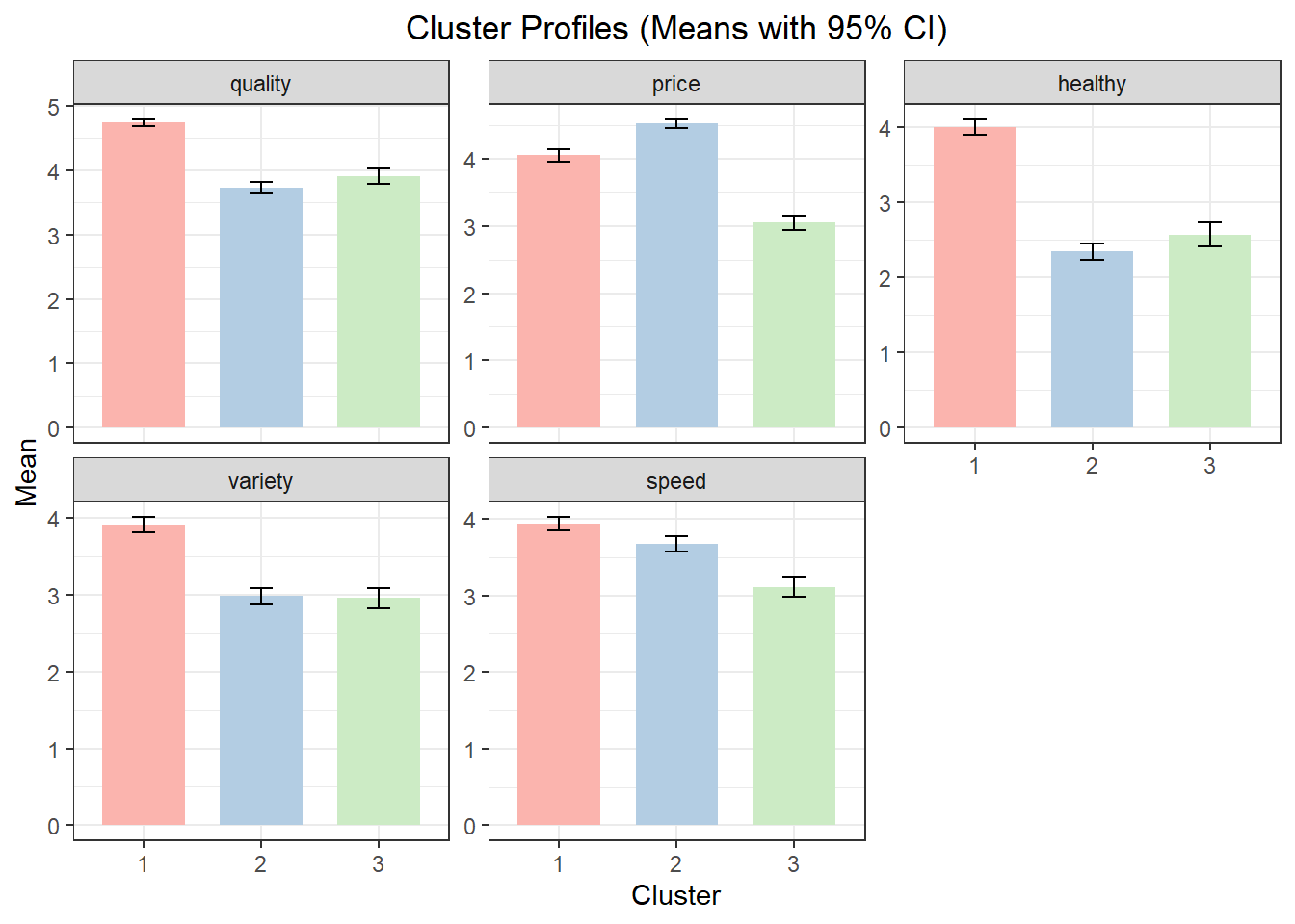

hc_final$plot

10.4 Describing and Labeling Hierarchical Clusters

Segmentation variables alone rarely provide enough context to understand who the clusters represent. Additional variables are used to describe and label the clusters. For both hierarchical clustering and k-means clustering (see below), use the easy_cluster_decribe() function from the MKT4320BGSU package to automate this process.

Usage:

easy_cluster_describe(data, cluster_col = "cluster", var, alpha = 0.05,
drop_missing = TRUE, auto_print = TRUE), digits = 4
where:
- data is the data frame containing the cluster membership column and variables to describe that was saved to the easy_hc_final object; should be objectname$data.
- cluster_col is a character string naming the cluster membership column in data (default = “cluster”).
- var is a character string naming the single variable to describe.
- alpha is the significance level for hypothesis tests (default = 0.05).
- drop_missing is logical; if TRUE (default), rows with missing cluster membership are dropped prior to analysis.
- auto_print is logical; if TRUE (default), prints summaries to the console; if FALSE returns results list
- digits is an integer for rounding/formatting of numeric output (default = 4).

Using the results from above (i.e., the hc_final$data object) , the output below highlights which variables significantly differentiate clusters and provides detailed summaries only where differences are statistically meaningful.

easy_cluster_describe(data = hc_final$data, cluster_col = "hc_cluster",
                      var="usertype")


Variable: usertype (categorical)

Overall test
Variable  Test        p_value  Significant
--------  ----------  -------  -----------
usertype  Chi-square  0.05500  FALSE      

Not significant at alpha = 0.05; no post-hoc shown.

easy_cluster_describe(data = hc_final$data, cluster_col = "hc_cluster",
                      var="spend")


Variable: spend (categorical)

Overall test
Variable  Test        p_value   Significant
--------  ----------  --------  -----------
spend     Chi-square  0.003500  TRUE       

Cross-tab (column %; clusters are columns)
Level         1      2      3    
------------  -----  -----  -----
$10 or more   25.25  17.48  26.63
$5 to $9      61.95  63.64  65.68
Less than $5  12.79  18.88  7.692

Post-hoc (Holm-adjusted p-values)
Row                       1:2      1:3     2:3     
------------------------  -------  ------  --------
$10 or more:$5 to $9      0.3758   1.000   0.5700  
$10 or more:Less than $5  0.06200  0.5700  0.002300
$5 to $9:Less than $5     0.5700   0.5700  0.03350

easy_cluster_describe(data = hc_final$data, cluster_col = "hc_cluster",
                      var="hours")


Variable: hours (continuous)

Overall test
Variable  Test   p_value  Significant
--------  -----  -------  -----------
hours     ANOVA  0        TRUE       

Cluster means (N, Mean, SD)
Cluster  N      Mean   SD    
-------  -----  -----  ------
1        297.0  3.710  0.9428
2        286.0  3.542  1.014 
3        169.0  3.065  1.070 

Significant differences: 1 > 3, 2 > 3

Post-hoc comparisons (Games-Howell)
.y.    group1  group2  estimate  conf.low  conf.high  p.adj            p.adj.signif
-----  ------  ------  --------  --------  ---------  ---------------  ------------
hours  1       2       -0.1685   -0.3592   0.02224    0.09600          ns          
hours  1       3       -0.6453   -0.8781   -0.4126    0.0000000007900  ****        
hours  2       3       -0.4769   -0.7166   -0.2372    0.00001220       ****

easy_cluster_describe(data = hc_final$data, cluster_col = "hc_cluster",
                      var="eatin")


Variable: eatin (continuous)

Overall test
Variable  Test   p_value  Significant
--------  -----  -------  -----------
eatin     ANOVA  0.02040  TRUE       

Cluster means (N, Mean, SD)
Cluster  N      Mean   SD   
-------  -----  -----  -----
1        297.0  3.986  2.000
2        286.0  4.441  1.978
3        169.0  4.160  1.903

Significant differences: 2 > 1

Post-hoc comparisons (Games-Howell)
.y.    group1  group2  estimate  conf.low  conf.high  p.adj    p.adj.signif
-----  ------  ------  --------  --------  ---------  -------  ------------
eatin  1       2       0.4540    0.06692   0.8411     0.01700  *           
eatin  1       3       0.1732    -0.2664   0.6129     0.6230   ns          
eatin  2       3       -0.2808   -0.7218   0.1602     0.2930   ns

easy_cluster_describe(data = hc_final$data, cluster_col = "hc_cluster",
                      var="mealplan")


Variable: mealplan (categorical)

Overall test
Variable  Test        p_value  Significant
--------  ----------  -------  -----------
mealplan  Chi-square  0.8882   FALSE      

Not significant at alpha = 0.05; no post-hoc shown.

easy_cluster_describe(data = hc_final$data, cluster_col = "hc_cluster",
                      var="gender")


Variable: gender (categorical)

Overall test
Variable  Test        p_value  Significant
--------  ----------  -------  -----------
gender    Chi-square  0        TRUE       

Cross-tab (column %; clusters are columns)
Level   1      2      3    
------  -----  -----  -----
Female  81.82  67.83  59.17
Male    18.18  32.17  40.83

Post-hoc (Holm-adjusted p-values)
Row          1:2        1:3  2:3    
-----------  ---------  ---  -------
Female:Male  0.0002000  0    0.06810

10.5 K-Means Clustering

10.5.1 Conceptual Overview

k-means clustering is a partition-based method that assigns observations to a fixed number of clusters by minimizing within-cluster variation. Unlike hierarchical clustering, k-means requires the analyst to specify the number of clusters in advance.

k-means is often preferred when:

Working with larger datasets
Refining a solution suggested by hierarchical clustering
Stability and computational efficiency are priorities

The process used for k-means clustering follows the process used above in hierarchical agglomerative clustering. That is, we first initially fit a number of potential solutions, and then we anlayze a final solution.

10.5.2 Initial K-Means Clustering Fit

We first fit k-means clustering solutions across a range of cluster counts using the easy_km_fit() function from the MKT4320BGSU package.

Usage:

easy_km_fit(data, vars, k_range = 1:10, standardize = TRUE, nstart = 25,
iter.max = 100, B = 20, seed = 4320)
where:
- data is a data frame containing the full dataset.
- vars is a character vector of numeric variable names used for clustering.
- k_range is an integer vector of cluster counts to evaluate (default = 1:10; allowed values 1–20).
- standardize is logical; if TRUE (default), clustering variables are standardized before fitting k-means.
- nstart is an integer; number of random starts for each k-means solution (default = 25).
- iter.max is an integer; maximum number of iterations allowed for each k-means run (default = 100).
- B is an integer; number of Monte Carlo bootstrap samples used to compute the Gap statistic (default = 20).
- seed is an integer; random seed for reproducible results (default = 4320).

We now fit the same variables we used above in hierarchical clustering. As before, the results should be saved to an object. The $diag diagnostics table saved in the object provides the necessary results to help decide on a (potential) final solution. The diagnostics table summarizes multiple stopping rules and balance checks across different values of $k$. No single statistic should be used in isolation when choosing the number of clusters. You can also view the $size_prop table to see the cluster sizes for all potential solutions.

km_vars <- c("quality", "price", "healthy", "variety", "speed")
km_fit <- easy_km_fit(data = ffseg, vars = km_vars, k_range = 2:8)
km_fit$diag

K-Means Cluster Diagnostics (Standardized)
Clusters	Silhouette	Gap.Stat	Small.Prop	Large.Prop	CV
2	0.2120	0.6307	0.4761	0.5239 ◊	0.068 *
3	0.1973	0.6150	0.2739	0.4096	0.208 *
4	0.1610	0.5953	0.2168	0.2806	0.105 *
5	0.1679	0.5855	0.1569	0.2340	0.178 *
6	0.1719	0.5827	0.1303	0.2354	0.224 *
7	0.1803	0.5741	0.1184	0.1835	0.195 *
8	0.1804	0.5747	0.0851	0.1582	0.185 *
^ Smallest cluster < 5% of sample.
◊ Largest cluster > 50% of sample.
* CV < 0.5 well balanced; ** moderately imbalanced.

km_fit$size_prop

Cluster Size Proportions by Solution
Solution	Cluster 1	Cluster 2	Cluster 3	Cluster 4	Cluster 5	Cluster 6	Cluster 7	Cluster 8
2-cluster solution	0.4761	0.5239
3-cluster solution	0.3165	0.4096	0.2739
4-cluster solution	0.2168	0.2487	0.2540	0.2806
5-cluster solution	0.2128	0.1569	0.2340	0.2287	0.1676
6-cluster solution	0.1423	0.1503	0.1303	0.1715	0.1702	0.2354
7-cluster solution	0.1263	0.1184	0.1516	0.1835	0.1769	0.1210	0.1223
8-cluster solution	0.1330	0.1436	0.1396	0.1582	0.1117	0.0851	0.1157	0.1130

10.5.3 Final K-Means Clustering Solution

After selecting a value for $k$, we finalize the k-means solution using the easy_km_final() function from the MKT4320BGSU package.

Usage:

easy_km_final(fit, data, k, cluster_col = "cluster", conf_level = 0.95, auto_print = TRUE)
where:
- fit is an object returned by easy_km_fit().
- data is the original full dataset used in easy_km_fit().
- k is an integer; number of clusters to extract.
- cluster_col is a character string; name of the cluster column to append to data (default = “cluster”).
- conf_level is numeric; confidence level for CI error bars (default = 0.95).
- auto_print is logical; if TRUE (default), prints selected outputs and displays the plot when the function is run.

km_final <- easy_km_final(fit = km_fit, data = ffseg, k = 3, 
                          cluster_col = "km_cluster", auto_print = FALSE)
km_final$props

  Cluster   N      Prop
1       1 238 0.3164894
2       2 308 0.4095745
3       3 206 0.2739362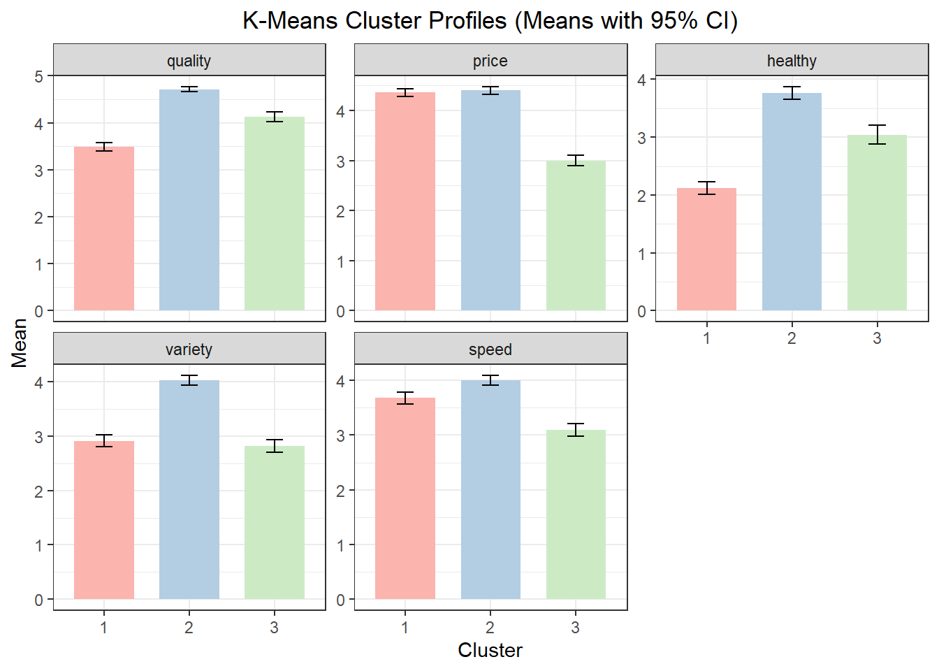

km_final$plot

km_final$profile

  Cluster  quality    price  healthy  variety    speed
1       1 3.483193 4.361345 2.117647 2.907563 3.680672
2       2 4.714286 4.399351 3.762987 4.022727 4.000000
3       3 4.131068 3.000000 3.043689 2.815534 3.097087

10.6 Describing and Labeling k-Means Clusters

As with hierarchical clustering, segmentation variables alone rarely provide enough context to understand who the clusters represent. Additional variables are used to describe and label the clusters. As with hierarchical clustering, use the easy_cluster_decribe() function from the MKT4320BGSU package to automate this process. See Section 10.4

10.7 Comparing Clustering Approaches

Hierarchical and k-means clustering often produce similar but not identical segmentation results. Differences between solutions can be informative and may reveal alternative ways to think about the market.

In practice, analysts often:

Use hierarchical clustering to explore the structure of the data
Use k-means clustering to refine and stabilize the final solution

10.8 Chapter Summary

In this chapter, we:

Introduced cluster analysis as a tool for marketing segmentation
Applied hierarchical and k-means clustering to the ffseg dataset
Used diagnostics to guide the choice of the number of clusters
Described and interpreted clusters in a marketing context

10.9 What’s Next

In the next chapter, we shift from grouping customers to summarizing and visualizing variables. Specifically, we will introduce Principal Components Analysis (PCA) and then extend it to PCA perceptual maps. PCA is a dimensionality-reduction technique that helps simplify complex datasets by transforming many correlated variables into a smaller set of components that capture the most important patterns in the data.

You will learn how PCA can be used to:

Reduce a large set of variables into a smaller number of interpretable dimensions
Identify underlying structures in consumer perceptions and evaluations
Prepare data for visualization and communication

We will then use these components to create perceptual maps, which are widely used in marketing to:

Visualize brand or product positions
Understand competitive structure
Support positioning and differentiation decisions

Chapter 10 Cluster Analysis

10.1 Why Cluster Analysis Matters in Marketing

10.2 The ffseg Dataset

10.3 Hierarchical Agglomerative Clustering

10.3.1 Conceptual Overview

10.3.2 Initial Hierarchical Clustering Fit

10.3.3 Selecting the Number of Clusters

10.3.4 Final Hierarchical Clustering Solution

10.4 Describing and Labeling Hierarchical Clusters

10.5 K-Means Clustering

10.5.1 Conceptual Overview

10.5.2 Initial K-Means Clustering Fit

10.5.3 Final K-Means Clustering Solution

10.6 Describing and Labeling k-Means Clusters

10.7 Comparing Clustering Approaches

10.8 Chapter Summary

10.9 What’s Next

10.2 The `ffseg` Dataset