Chapter 13 Standard Multinomial Logit Models

13.1 Introduction to Multinomial Choice in Marketing

Many marketing decisions involve choices among more than two discrete alternatives. Consumers may choose among competing brands, subscription plans, service providers, or product variants. When the outcome variable has more than two unordered categories, linear regression and binary logistic regression are no longer appropriate.

The standard multinomial logit (MNL) model is the most common baseline model for analyzing and predicting such outcomes. In marketing analytics, it is widely used for brand choice, product selection, and competitive response analysis. The focus of this chapter is on applied interpretation rather than mathematical derivation.

13.2 The `bfast` Dataset

In this chapter, we use the bfast dataset, which contains data on breakfast food preferences. Each observation represents a consumer choice occasion in which one type of food was selected from a competitive set.

The outcome variable records the chosen type, while predictor variables capture marketing mix and consumer characteristics that may influence choice. Our core marketing question is: Which factors increase or decrease the probability that a consumer chooses a particular fast-food brand?

13.3 Training and Test Samples

To evaluate predictive performance, we split the data into training and test samples. As with binary logistic regression, we use the splitsample() function from the MKT4320BGSU package. This function creates reproducible partitions and supports stratification on the outcome variable.

Usage:

splitsample(data, outcome = NULL, group = NULL, choice = NULL, alt = NULL,
p = 0.75, seed = 4320)
where:
- data is the data frame to split.
- outcome is the outcome variable in quotes used for stratification. Required when group is NULL. Optional when group is provided. For standard MNL, it is required.
- group is NOT USED FOR STANDARD MNL
- choice is NOT USED FOR STANDARD MNL
- alt is NOT USED FOR STANDARD MNL
- p is the proportion of observations to place in the training set. Must be strictly between 0 and 1. Default is 0.75.
- seed is the random seed for reproducibility. Default is 4320.

Below, we create are training and test samples. We also check the outcome variable in the two samples to ensure they are similar proportions in each.

sp <- splitsample(data = bfast, outcome = "bfast")
train <- sp$train
test  <- sp$test

proportions(table(train$bfast))


   Cereal       Bar   Oatmeal 
0.3851964 0.2628399 0.3519637

proportions(table(test$bfast))


   Cereal       Bar   Oatmeal 
0.3853211 0.2614679 0.3532110

13.4 Estimating a Standard Multinomial Logit Model

We estimate the standard multinomial logit model using nnet::multinom(). It is important to include model = TRUE so that model diagnostics and classification results can be computed later.

Using the summary() function in base R will provide the raw coefficients from the model. The estimated coefficients describe how each predictor affects the relative log-odds of choosing one product versus the reference product.

library(nnet)
mnl_fit <- multinom(bfast ~ gender + marital + lifestyle + age, 
                    model = TRUE, data=train)

# weights:  18 (10 variable)
initial  value 727.281335 
iter  10 value 579.014122
final  value 574.997631 
converged

summary(mnl_fit)

Call:
multinom(formula = bfast ~ gender + marital + lifestyle + age, 
    data = train, model = TRUE)

Coefficients:
        (Intercept)  genderMale maritalUnmarried lifestyleInactive         age
Bar       0.8832457 -0.21298963        0.6126977        -0.7865772 -0.02532866
Oatmeal  -4.4920408 -0.02262325       -0.3897362         0.3187473  0.07996475

Std. Errors:
        (Intercept) genderMale maritalUnmarried lifestyleInactive         age
Bar       0.3256994  0.2064320        0.2123832         0.2090460 0.006655803
Oatmeal   0.4596750  0.2094666        0.2366511         0.2156992 0.007755708

Residual Deviance: 1149.995 
AIC: 1169.995

13.5 Evaluating Model Fit

Raw coefficients alone do not indicate whether a model performs well. We use eval_std_mnl() from the MKT4320BGSU package to compute model-fit statistics and diagnostics.

Usage:

eval_std_mnl(OBJ, exp = FALSE, digits = 4, ft = FALSE, newdata = NULL,
label_model = "Model data", label_newdata = "New data", class_digits = 3)
where:
- model is a fitted multinom model.
- exp is logical; if TRUE, return relative risk ratios (exp(beta)). If FALSE, return log-odds coefficients (default = FALSE).
- digits is an integer; number of decimals used to round coefficient and model-fit results (default = 4).
- ft is logical; if TRUE, return coefficient and classification tables as flextable objects (default = FALSE).
- newdata is an optional data frame for an additional classification matrix (e.g., a holdout or test set). If NULL, only the model-data classification is produced.
- label_model is a character string; label for the model-data classification output (default = “Model data”).
- label_newdata is a character string; label for the newdata classification output (default = “New data”).
- class_digits is an integer; number of decimals used to round classification statistics (default = 3).

Key outputs include:

A likelihood-ratio test comparing the fitted model to an intercept-only model
McFadden’s pseudo R-squared
Classification accuracy and diagnostics

In applied marketing contexts, even modest pseudo R-squared values can indicate meaningful improvements over random choice.

mnl_eval <- eval_std_mnl(model = mnl_fit, newdata = test, ft = TRUE)
mnl_eval

LR chi2 (8) = 288.1568; p < 0.0001
McFadden's Pseudo R-square = 0.2004
y.level	term	logodds	std.error	statistic	p.value
Bar	(Intercept)	0.8832	0.3257	2.7118	0.0067
Bar	genderMale	-0.2130	0.2064	-1.0318	0.3022
Bar	maritalUnmarried	0.6127	0.2124	2.8849	0.0039
Bar	lifestyleInactive	-0.7866	0.2090	-3.7627	0.0002
Bar	age	-0.0253	0.0067	-3.8055	0.0001
Oatmeal	(Intercept)	-4.4920	0.4597	-9.7722	0.0000
Oatmeal	genderMale	-0.0226	0.2095	-0.1080	0.9140
Oatmeal	maritalUnmarried	-0.3897	0.2367	-1.6469	0.0996
Oatmeal	lifestyleInactive	0.3187	0.2157	1.4777	0.1395
Oatmeal	age	0.0800	0.0078	10.3104	0.0000

Classification Matrix - Model data
Accuracy = 0.562
PCC = 0.341
	Reference
Predicted	Cereal	Bar	Oatmeal	Total
Cereal	124	85	46	255
Bar	52	68	7	127
Oatmeal	79	21	180	280
Total	255	174	233	662
Statistics by Class:
Sensitivity	0.486	0.391	0.773
Specificity	0.678	0.879	0.767
Precision	0.486	0.535	0.643

Classification Matrix - New data
Accuracy = 0.583
PCC = 0.342
	Reference
Predicted	Cereal	Bar	Oatmeal	Total
Cereal	45	24	20	89
Bar	18	25	0	43
Oatmeal	21	8	57	86
Total	84	57	77	218
Statistics by Class:
Sensitivity	0.536	0.439	0.740
Specificity	0.672	0.888	0.794
Precision	0.506	0.581	0.663

13.5.1 Interpreting Coefficients

Coefficient estimates in a standard MNL model are interpreted relative to the reference brand. A positive coefficient means that higher values of the predictor increase the likelihood of choosing that brand relative to the baseline.

To aid interpretation, coefficients can also be expressed as relative risk ratios (RRRs). RRRs greater than 1 indicate increased relative likelihood, while values below 1 indicate decreased likelihood. These interpretations are often more intuitive for managerial audiences.

mnl_eval_rrr <- eval_std_mnl(model = mnl_fit, exp = TRUE, 
                             newdata = test, ft=TRUE)
mnl_eval_rrr$coef_table

LR chi2 (8) = 288.1568; p < 0.0001
McFadden's Pseudo R-square = 0.2004
y.level	term	RRR	std.error	statistic	p.value
Bar	(Intercept)	2.4187	0.3257	2.7118	0.0067
Bar	genderMale	0.8082	0.2064	-1.0318	0.3022
Bar	maritalUnmarried	1.8454	0.2124	2.8849	0.0039
Bar	lifestyleInactive	0.4554	0.2090	-3.7627	0.0002
Bar	age	0.9750	0.0067	-3.8055	0.0001
Oatmeal	(Intercept)	0.0112	0.4597	-9.7722	0.0000
Oatmeal	genderMale	0.9776	0.2095	-0.1080	0.9140
Oatmeal	maritalUnmarried	0.6772	0.2367	-1.6469	0.0996
Oatmeal	lifestyleInactive	1.3754	0.2157	1.4777	0.1395
Oatmeal	age	1.0832	0.0078	10.3104	0.0000

13.5.2 Classification Performance

Beyond fit statistics, classification results help assess how well the model predicts observed choices.

The output includes:

Overall accuracy
Proportional Chance Criterion (PCC)
Product-specific sensitivity, specificity, and precision

These metrics help identify which brands are easier or harder to predict based on observed covariates.

13.5.3 Holdout Sample Evaluation

Evaluating the model on a test sample provides insight into how well it generalizes to new data. Large discrepancies between training and test performance may indicate overfitting.

In practice, marketing data often contain substantial noise, so perfect prediction is neither expected nor required for managerial usefulness.

13.6 Predicted Probabilities

Coefficients and classification tables are not always the most intuitive outputs for decision-makers. Predicted probabilities translate model results into directly interpretable quantities.

We use the pp_std_mnl() function from the MKT4320BGSU package to compute and visualize average predicted probabilities for a focal predictor.

Usage:

pp_std_mnl(model, focal, interaction = NULL, xlab = NULL, ft_table = TRUE)
where:
- model is a fitted multinom model.
- focal is a character string; name of the focal predictor variable.
- interaction is an optional character string giving a giving a factor variable used for interaction plots.
- xlab is an optional character string; label for the x-axis in the plot.
- ft_table is logical; if TRUE, return the probability table as a flextable (default = TRUE).

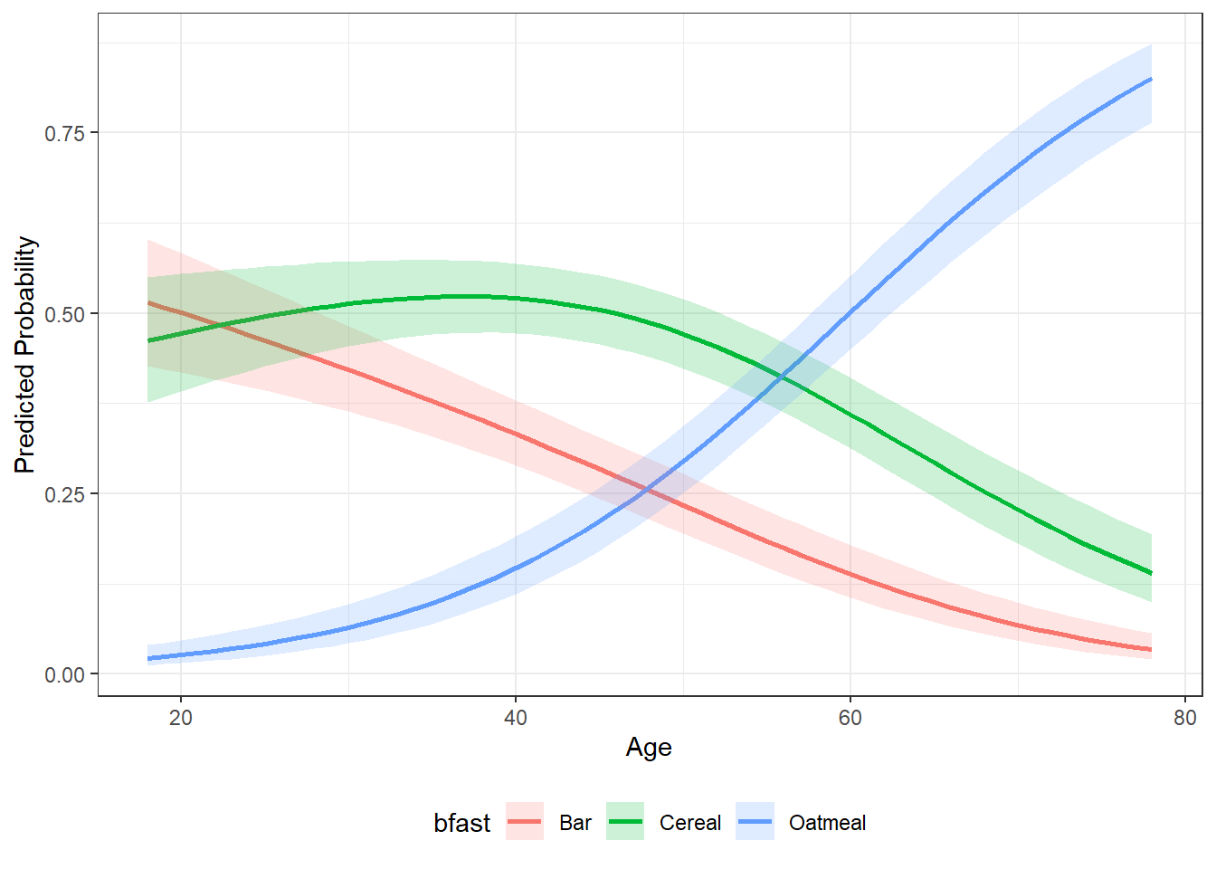
13.6.1 Continuous Focal Variable

For a numeric focal predictor, the function produces:

a smooth probability curve across the observed range of the variable
a compact table showing predicted probabilities at:
- one standard deviation below the mean, the mean, and one standard deviation above the mean

pp_age <- pp_std_mnl(model = mnl_fit, focal = "age", xlab  = "Age")
pp_age$table

age	bfast	p.prob	lower.CI	upper.CI
31.05	Cereal	0.5160	0.4588	0.5727
31.05	Bar	0.4130	0.3570	0.4713
31.05	Oatmeal	0.0711	0.0475	0.1050
48.91	Cereal	0.4799	0.4321	0.5281
48.91	Bar	0.2443	0.2052	0.2883
48.91	Oatmeal	0.2757	0.2323	0.3239
66.76	Cereal	0.2689	0.2212	0.3227
66.76	Bar	0.0871	0.0617	0.1217
66.76	Oatmeal	0.6440	0.5852	0.6987

pp_age$plot

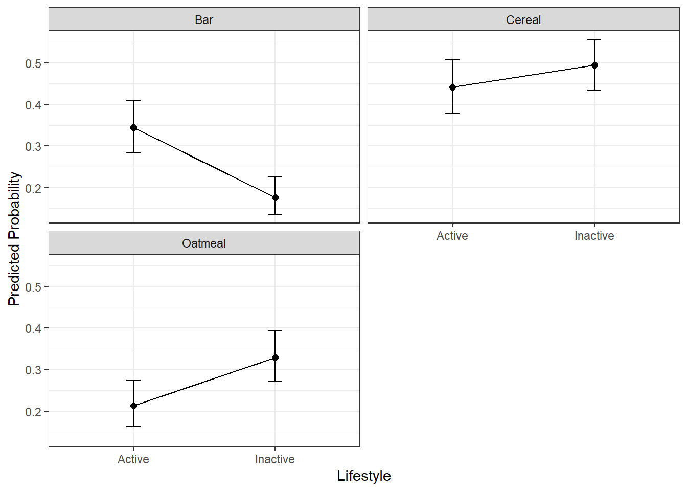
13.6.2 Categorical Focal Variable

For a factor focal predictor, predicted probabilities are computed across all levels of the variable.

pp_lifestyle <- pp_std_mnl(model = mnl_fit, focal= "lifestyle", 
                           xlab = "Lifestyle")
pp_lifestyle$table

lifestyle	bfast	p.prob	lower.CI	upper.CI
Active	Cereal	0.4417	0.3784	0.5070
Active	Bar	0.3450	0.2849	0.4104
Active	Oatmeal	0.2133	0.1624	0.2750
Inactive	Cereal	0.4951	0.4347	0.5555
Inactive	Bar	0.1761	0.1351	0.2263
Inactive	Oatmeal	0.3289	0.2711	0.3923

pp_lifestyle$plot

13.6.3 Continuous by Categorical Interaction

When a factor interaction variable is supplied, predicted probabilities are shown separately for each interaction level, which is especially useful when examining whether the effect of a numeric predictor differs across groups. In interaction plots:

the continuous focal variable remains on the x-axis
separate lines represent levels of the categorical interaction variable
panels show predicted probabilities for each outcome category

mnl_fit_int <- multinom(bfast ~ gender + marital + lifestyle*age,
                        model = TRUE, data=train)

# weights:  21 (12 variable)
initial  value 727.281335 
iter  10 value 585.939749
iter  20 value 573.009001
final  value 573.008988 
converged

pp_int <- pp_std_mnl(model = mnl_fit_int, focal="age", 
                     interaction = "lifestyle", xlab = "Age")
pp_int$plot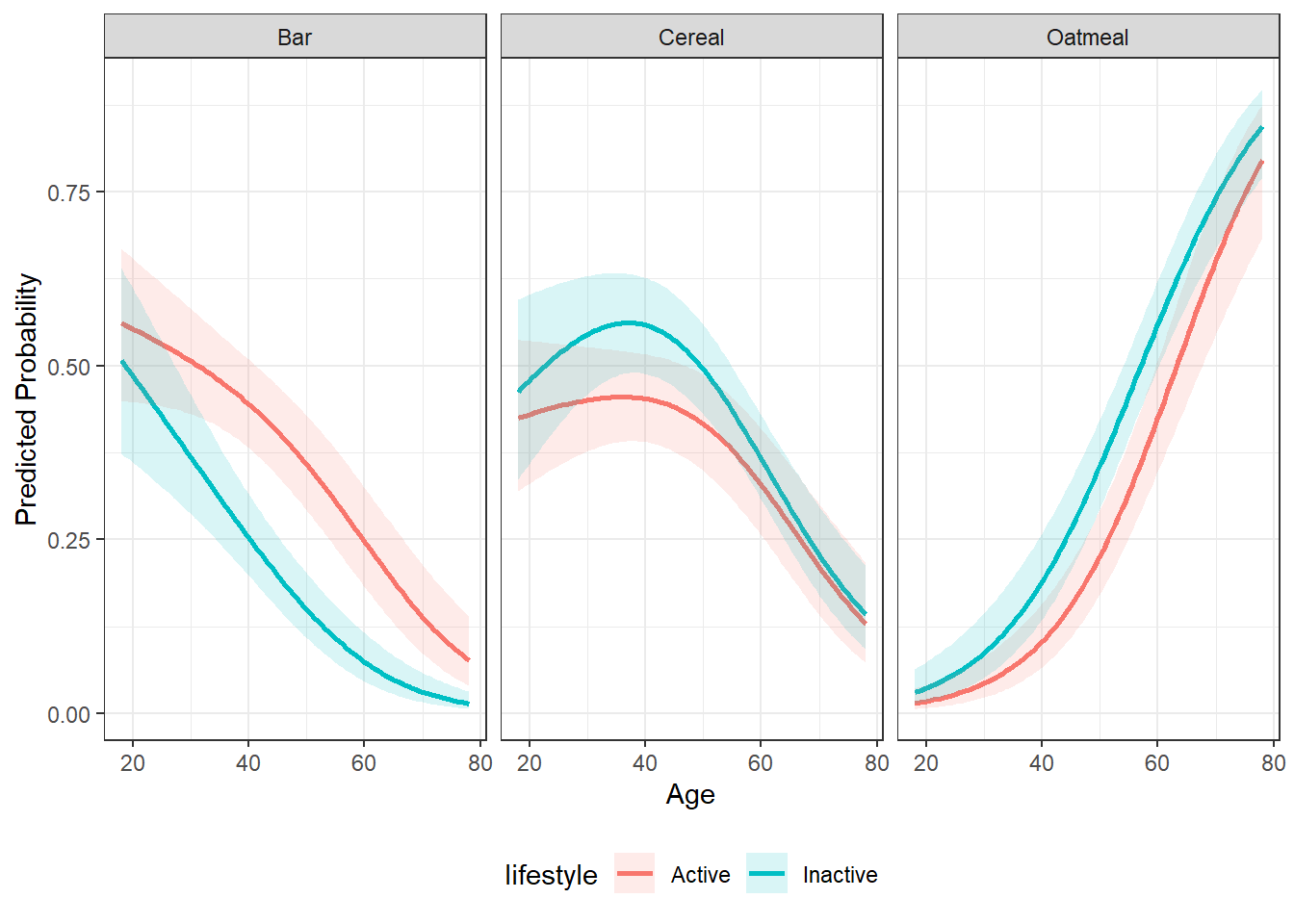

Predicted probabilities help answer questions such as:

How does increasing price shift brand choice probabilities?
Which brands are most sensitive to changes in a predictor?
Does the effect of one variable differ across groups?

Because multinomial probabilities must sum to 1, an increase in one brand’s probability often reflects substitution away from another brand rather than a direct increase in preference.

13.7 Marketing Interpretation

The standard multinomial logit model provides a powerful yet accessible framework for understanding brand choice. It allows marketers to:

Compare competitive positioning across brands
Assess price and promotion sensitivity
Translate statistical estimates into actionable probabilities

However, it also has limitations, including restrictive substitution patterns across alternatives.

13.8 Summary

In this chapter, you learned how to:

Estimate a standard multinomial logit model
Evaluate model fit and predictive performance
Interpret coefficients and relative risk ratios
Use predicted probabilities for marketing insight

The standard MNL model serves as a foundational tool in marketing analytics and provides a benchmark against which more advanced choice models can be compared.

13.9 What’s Next

In this chapter, we treated brand choice as a function of consumer-level characteristics and marketing variables that affect all alternatives in the same way. This approach works well as a baseline, but it imposes an important limitation: it assumes that predictors influence every brand symmetrically.

In the next chapter, we relax this restriction by introducing the alternative-specific multinomial logit (AS-MNL) model. This framework allows predictors—such as price, promotions, or product attributes—to vary by brand, more closely reflecting how consumers actually evaluate competing options.

You will learn how to: - Specify predictors that differ across alternatives - Interpret coefficients that are specific to each brand - Compare alternative-specific results to the standard MNL model - Gain deeper insight into competitive positioning and substitution patterns

Alternative-specific MNL models provide a major step forward in realism and interpretability, especially in marketing settings where attributes like price, availability, or features differ meaningfully across brands.

Chapter 13 Standard Multinomial Logit Models

13.1 Introduction to Multinomial Choice in Marketing

13.2 The bfast Dataset

13.3 Training and Test Samples

13.4 Estimating a Standard Multinomial Logit Model

13.5 Evaluating Model Fit

13.5.1 Interpreting Coefficients

13.5.2 Classification Performance

13.5.3 Holdout Sample Evaluation

13.6 Predicted Probabilities

13.6.1 Continuous Focal Variable

13.6.2 Categorical Focal Variable

13.6.3 Continuous by Categorical Interaction

13.7 Marketing Interpretation

13.8 Summary

13.9 What’s Next

13.2 The `bfast` Dataset