Chapter 10 Alt-Specific MNL

Data for this chapter:

The train.yog and test.yog data are used from the MKT4320BGSU course package. Load the package and use the data() function to load the data.
```
# Load the course package
library(MKT4320BGSU)
# Load the data
data(train.yog)
data(test.yog)
```

10.1 Introduction

Base R is not good for alternative specific multinomial logistic regression (MNL). The best package that I have found for alternative specific MNL is mlogit with its mlogit function. Use install.packages("mlogit") to install the package on your machine, then load it using the library function when needed.

library(mlogit)

However, even that is not very user friendly (in my opinion). Therefore, I have written a few user defined functions to help with getting the necessary results from an alternative specific MNL. * asmnl_est produces Odds Ratio coefficients table, overall model significance, McFadden’s Pseudo-\(R^2\), and classification matrices for both the training data and the test/holdout data * asmnl_me produces marginal effects tables for all IVs * asmnl_mp produces margin plots for case-specific IVs

10.2 Alt-Spec MNL using User Defined Function

Alternative Specific MNL is performed using the asmnl_est user defined function
Usage: asmnl_est(formula, data, id="", alt="", choice="", testdata)
- formula is an object with a saved formula. The formula is represented by a DV on the left side separated from the IVs on the right side by a tilde(~). The IVs are further separated by having choice-specific variables on the left and the case-specific variables on the right, separated by a vertical line, |. For example:
  - myform = choice ~ chvar1 + chvar2 | casvar1 + casvar2
- data is the name of the training data
- id is the variable that identifies the case (in quotes)
- alt is the variable that identifies the choice (in quotes)
- choice is the variable that identifies if alt was selected or not
- testdata is the name of the test data
The function will display the coefficients table, overall model significance, McFadden’s Pseudo-\(R^2\), and classification matrices for both the training data and the test/holdout data
In addition, the results should be saved to an object to be used in other user defined functions
NOTE 1: To work properly, all factor IVs should already be in dummy variable coding
NOTE 2: This function also requires the broom package

library(mlogit)
# Saving formula to object
myform <- choice ~ feat + price | income

asmod <- asmnl_est(formula=myform,
               data=train.yog,
               id="id",
               alt="brand",
               choice="choice",
               testdata=test.yog)



---------
Model Fit
---------

Log-Likelihood: -1618.4208
McFadden R^2: 0.2397
Likelihood ratio test: chisq = 1020.5649 (p.value < .0001)

---------------------
OR Estimation Results
---------------------

                term estimate std.error statistic p.value
  (Intercept):Hiland   2.1355    0.5677    1.3365  0.1814
  (Intercept):Weight   0.9740    0.2079   -0.1269  0.8990
 (Intercept):Yoplait   0.0185    0.2680  -14.8845  0.0000
                feat   1.5267    0.1491    2.8371  0.0046
               price   0.6425    0.0296  -14.9691  0.0000
       income:Hiland   0.8975    0.0149   -7.2464  0.0000
       income:Weight   0.9886    0.0038   -3.0436  0.0023
      income:Yoplait   1.0756    0.0040   18.1030  0.0000

---------------------------------------
Classification Matrix for Training Data
---------------------------------------
0.6207 = Hit Ratio
0.3299 = PCC

          T.Dannon T.Hiland T.Weight T.Yoplait Total
P.Dannon       577       39      324        97  1037
P.Hiland         1       12        0         2    15
P.Weight        18        2       38        18    76
P.Yoplait      132        1       53       497   683
Total          728       54      415       614  1811

--------------------------------------
Classification Matrix for Holdout Data
--------------------------------------
0.6073 = Hit Ratio
0.3309 = PCC

          T.Dannon T.Hiland T.Weight T.Yoplait Total
P.Dannon       199       14      104        38   355
P.Hiland         2        2        1         1     6
P.Weight         8        1       12        13    34
P.Yoplait       33        0       21       152   206
Total          242       17      138       204   601

10.2.1 Marginal Effects

The asmnl_me user defined function will be used to get the marginal effects of the IVs
Usage: asmnl_me(mod)
- mod is the object containing the result of the mlogit call using the asmnl_est user defined function

asmnl_me(asmod)


--------------------------------
Predicted Probabilities at Means
--------------------------------
 Dannon  Hiland  Weight Yoplait 
 0.4832  0.0048  0.2571  0.2549 

 ------------------------- 
 Marginal effects for feat 
 ------------------------- 
          Dannon   Hiland   Weight  Yoplait
Dannon   0.10565 -0.00098 -0.05256 -0.05212
Hiland  -0.00098  0.00201 -0.00052 -0.00052
Weight  -0.05256 -0.00052  0.08080 -0.02773
Yoplait -0.05212 -0.00052 -0.02773  0.08036

 -------------------------- 
 Marginal effects for price 
 -------------------------- 
          Dannon   Hiland   Weight  Yoplait
Dannon  -0.11049  0.00102  0.05496  0.05450
Hiland   0.00102 -0.00211  0.00054  0.00054
Weight   0.05496  0.00054 -0.08450  0.02899
Yoplait  0.05450  0.00054  0.02899 -0.08404

 --------------------------- 
 Marginal effects for income 
 --------------------------- 
  Dannon   Hiland   Weight  Yoplait 
-0.00731 -0.00059 -0.00684  0.01473

10.2.2 Margin Plots

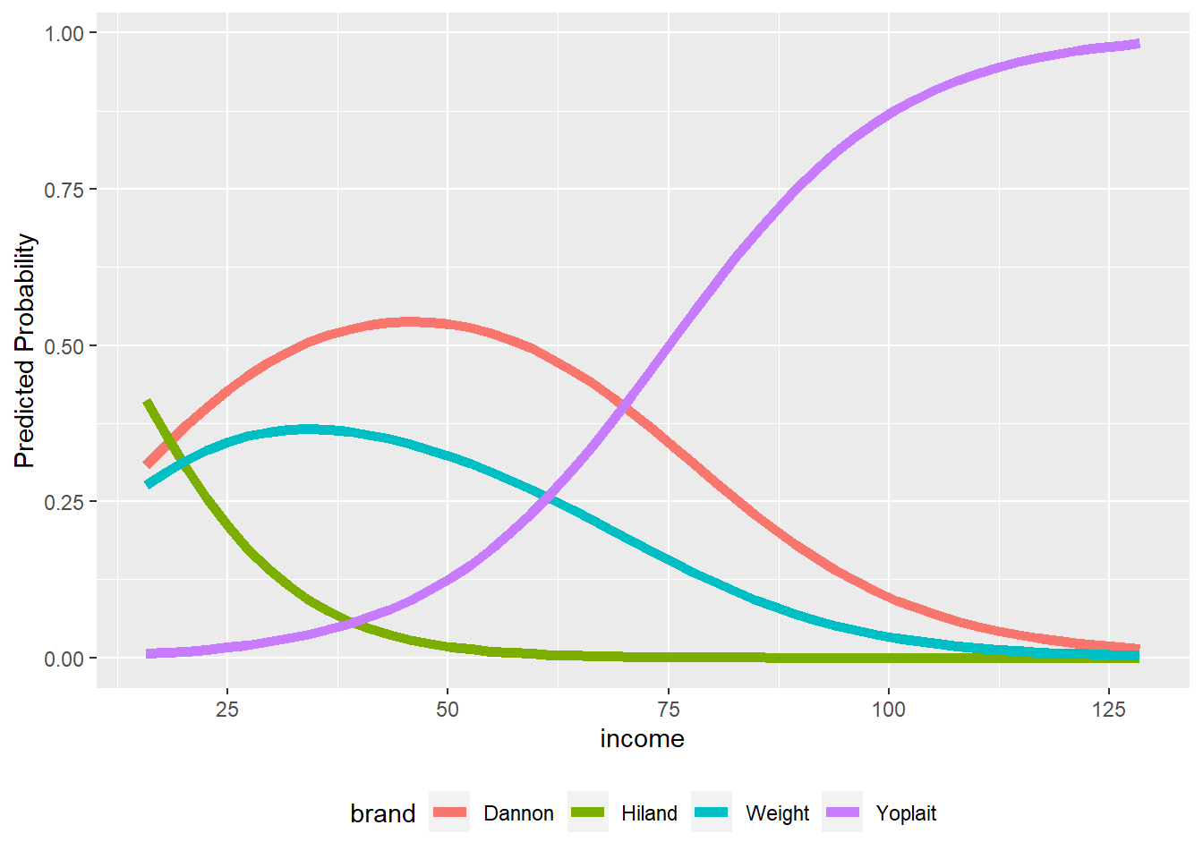
The asmnl_mp user defined function will create margin plots for a case-specific IV
Usage: almnl_mp(mod, focal="", type="") *modis the object containing the result of themlogitcall using theasmnl_estuser defined function *focalis the case-specific IV for which a margin plot is wanted (in quotes) *typeis the type of IV; must be either“C”for continuous or“D”` for dummy
NOTE: This function requires the ggplot2 package

asmnl_mp(asmod,"income", "C")