Chapter 4 Logistic Regression (Binary)

Sources for this chapter:

R for Marketing Research ad Analytics, Second Edition (2019). Chris Chapman and Elea McDonnell Feit
- http://r-marketing.r-forge.r-project.org/index.html
ggplot2: https://ggplot2.tidyverse.org/

Data for this chapter:

The directmktg data is used from the MKT4320BGSU course package. Load the package and use the data() function to load the data.
```
# Load the course package
library(MKT4320BGSU)
# Load the data
data(directmktg)
```

4.1 Introduction

Base R is typically sufficient for performing the basics of logisitic regression, but to get some of the outputs required, I have created some user defined functions that are available in the course package.

or_table.R() produces Odds Ratio Coefficients
logreg_cm() produces the Classification Matrix
logreg_roc() produces the ROC Curves
gainlift() produces Gain/Lift tables and charts
logreg_cut() produces the Sensitivity/Specificity Plot

Video Tutorial: Logistic Regression - Introduction

4.2 The `glm()` Function

glm stands for Generalized Linear Model, and this function can be used with a variety of dependent variables by specifying different family="FAMILY" options *lm(dv ~ iv1 + iv2, data) is the same as
`glm(dv ~ iv1 + iv2, data, family=“gaussian”)
Usage: glm(formula, data, family)

4.3 Logistic Regression using `glm()`

Binary logistic regression is performed using the glm() function when the family="binomial" is specified.
Usage: glm(formula, data, family="binonmial")
- family="binomial" tells R to use logistic regression on a binary dependent variable

If glm(formula, data, family="binomial") is run by itself, R only outputs the **Logit formulation* coefficients (and some other measures)

glm(buy ~ age + gender, directmktg, family="binomial")


Call:  glm(formula = buy ~ age + gender, family = "binomial", data = directmktg)

Coefficients:
 (Intercept)           age  genderFemale  
    -8.02069       0.18954      -0.09468  

Degrees of Freedom: 399 Total (i.e. Null);  397 Residual
Null Deviance:      521.6 
Residual Deviance: 336.1    AIC: 342.1

Table 4.1: Logit Coefficients from glm() call

Video Tutorial: glm() Basic Usage

However, if the results of the glm() call are assigned to an object, the Base R summary() function can be used to get much more detailed output, but requires manual calculation of McFadden’s Pseudo-$R^2$

prelim <- glm(buy ~ age + gender, directmktg, family="binomial")
summary(prelim)


Call:
glm(formula = buy ~ age + gender, family = "binomial", data = directmktg)

Coefficients:
             Estimate Std. Error z value Pr(>|z|)    
(Intercept)  -8.02069    0.78700 -10.191   <2e-16 ***
age           0.18954    0.01926   9.842   <2e-16 ***
genderFemale -0.09468    0.27354  -0.346    0.729    
---
Signif. codes:  0 '***' 0.001 '**' 0.01 '*' 0.05 '.' 0.1 ' ' 1

(Dispersion parameter for binomial family taken to be 1)

    Null deviance: 521.57  on 399  degrees of freedom
Residual deviance: 336.14  on 397  degrees of freedom
AIC: 342.14

Number of Fisher Scoring iterations: 5

# Manually calculate McFadden's Pseudo R-sq
Mrsq <- 1-prelim$deviance/prelim$null.deviance
cat("McFadden's Pseudo-Rsquared = ", Mrsq)

McFadden's Pseudo-Rsquared =  0.3555239

Table 4.2: Summary results from glm() call

Video Tutorial: glm() Output

For “nicer” looking results, the package jtools can be used

library(jtools)
summ(prelim,   # Saved object from before
     digits=4, # How many digits to display in each column
     model.info = FALSE)  # Suppress extraneous information

χ²(2)	185.4317
Pseudo-R² (Cragg-Uhler)	0.5092
Pseudo-R² (McFadden)	0.3555
AIC	342.1413
BIC	354.1157

	Est.	S.E.	z val.	p
(Intercept)	-8.0207	0.7870	-10.1915	0.0000
age	0.1895	0.0193	9.8422	0.0000
genderFemale	-0.0947	0.2735	-0.3461	0.7293
Standard errors: MLE

Table 4.3: Summary results from glm() using jtools package

Video Tutorial: glm() Output Using the jtools Package

4.3.1 Odds Ratio Coefficients

To get the Odds Ratio coefficients, use the or_table() function from the MKT4320BGSU course package.

Usage: or_table(MODEL, DIGITS, CONF)

MODEL is the name of the object with results of the glm() call
DIGITS is the number of digits to round the values to in the table
CONF is the confidence interval level (e.g., 95 = 95%)

or_table(prelim,  # Saved logistic regression model from above
             4,      # Number of digits to round output to
             95)    # Level of confidence

                Parameter OR Est      p   2.5%  97.5%
(Intercept)   (Intercept) 0.0003 0.0000 0.0001 0.0015
age                   age 1.2087 0.0000 1.1639 1.2552
genderFemale genderFemale 0.9097 0.7293 0.5322 1.5550

Table 4.4: Odds Ratio Coefficients

Odds Ratio coefficients can also be obtained from the summ function of the jtools package

summ(prelim,   # Saved object from before
     digits=4, # How many digits to display in each column
     exp = TRUE,  # Obtain exponentiated coefficients (i.e., Odds Ratio)
     model.info = FALSE)  # Suppress extraneous information

χ²(2)	185.4317
Pseudo-R² (Cragg-Uhler)	0.5092
Pseudo-R² (McFadden)	0.3555
AIC	342.1413
BIC	354.1157

	exp(Est.)	2.5%	97.5%	z val.	p
(Intercept)	0.0003	0.0001	0.0015	-10.1915	0.0000
age	1.2087	1.1639	1.2552	9.8422	0.0000
genderFemale	0.9097	0.5322	1.5550	-0.3461	0.7293
Standard errors: MLE

Table 4.5: Odds Ratio Coefficients using jtools package

Video Tutorial: glm() Odds Ratio Coefficients

4.4 Estimate with Training Sample Only

Generally, it is good practice to use a training sample and a testing/holdout sample to see how well the model performs “out of sample”. To do this, the data must be split into two groups: train and test

4.4.1 Creating `train` and `test` Samples

While this can be done in a number of ways, the package caret has a very useful function that attempts to balance the percent of “positive” cases in both samples, while still creating random samples
After running this procedure, two new data frames will be created
- One containing the training data, train
- One containing the testing/holdout data, test

Two methods are available: using the splitsample function from the MKT4320BGSU package or manually using caret

To use the splitsample function
- Usage: splitsample(data, outcome, p=0.75, seed=4320)
  - data is the name of the dataframe to be used to estimate the model
  - outcome is the name of the outcome variable (i.e., dependent variable) for the model to be estimated
  - p is the percent of the data to be assigned to the training sample; defaults to 0.75
  - seed is an integer to be used for random number generation; defaults to 4320
- Requires the caret package
- Will create two new dataframes in your environment: train and test

splitsample(directmktg, buy)

To use the caret package manually, follow the code below

# Use 'caret' package to create training and test/holdout samples
# This will create two separate dataframes: train and test

library(caret)    # Load the 'caret package'

# Start by setting a random number seed so that the same samples
# will be created each time
set.seed(4320)

# Create a dataframe of row numbers that should be in the 'train' sample
inTrain <- createDataPartition(y=directmktg$buy, # Outcome variable
                               p=.75, # Percent of sample to be in 'train'
                               list=FALSE)  # Put result in matrix

# Select only rows from data that are in 'inTrain'; assign to 'train'
train <- directmktg[inTrain,]
# Select only rows from data that not in 'inTrain'; assign to 'test'
test <- directmktg[-inTrain,]

Video Tutorial: Creating Training and Test Samples

4.4.2 Run Model with only Training Sample

Once completed, run the model on the training sample only

Goodness-of-Fit measures can be obtained from the results

model <- glm(buy ~ age + gender, train, family="binomial")
summ(model,   # 'jtools' results; use 'summary' for Base R
     4, model.info=FALSE)

χ²(2)	130.57
Pseudo-R² (Cragg-Uhler)	0.48
Pseudo-R² (McFadden)	0.33
AIC	268.37
BIC	279.49

	Est.	S.E.	z val.	p
(Intercept)	-7.71	0.87	-8.81	0.00
age	0.18	0.02	8.52	0.00
genderFemale	-0.01	0.31	-0.04	0.97
Standard errors: MLE; Continuous predictors are mean-centered and scaled by 1 s.d. The outcome variable remains in its original units.

or_table(model)

                Parameter OR Est     p   2.5%  97.5%
(Intercept)   (Intercept) 0.0004 0.000 0.0001 0.0025
age                   age 1.1996 0.000 1.1505 1.2509
genderFemale genderFemale 0.9873 0.967 0.5399 1.8056

Table 4.6: Logistic Regression Results for Training Sample

Video Tutorial: Model Fit - Goodness-of-Fit Measures

4.5 Classification Matrix

To get the Classification Matrix, use the logreg_cm() function from the MKT4320BGSU course package.
Usage: logreg_cm(MOD, DATA, "POS", CUTOFF=)
- MOD is the name of the object with results of the glm() call
- DATA is the data set for which the Classification Matrix should be produced (i.e., original, training, or testing)
- "POS" is the level of the factor variable that is the SUCCESS level
- CUTOFF= is the cutoff threshold; default is 0.5

This function requires the package caret, which should already be loaded from the splitting of the data

# Classification Matrix for training sample
logreg_cm(model,   # Name of the results object
          train,   # Use training sample
          "Yes")   # Level of 'buy' that represents success/true

Confusion Matrix and Statistics

          Reference
Prediction  No Yes
       No  179  37
       Yes  14  71

               Accuracy : 0.8306          
                 95% CI : (0.7833, 0.8712)
    No Information Rate : 0.6412          
    P-Value [Acc > NIR] : 3.179e-13       

                  Kappa : 0.6136          

 Mcnemar's Test P-Value : 0.002066        

            Sensitivity : 0.6574          
            Specificity : 0.9275          
         Pos Pred Value : 0.8353          
         Neg Pred Value : 0.8287          
             Prevalence : 0.3588          
         Detection Rate : 0.2359          
   Detection Prevalence : 0.2824          
      Balanced Accuracy : 0.7924          

       'Positive' Class : Yes             

PCC = 53.99%

Table 4.7: Classification Matrix for Training Sample

Video Tutorial: Model Fit - Classification Matrix

4.6 ROC Curve

To get the ROC curve, use the user defined function ``logreg_roc() function from the MKT4320BGSU course package.
Usage: logreg_roc(MOD, DATA)
- MOD is the name of the object with results of the glm() call
- DATA is the data set for which the ROC should be produced (i.e., original, training, or testing)

This function requires the package pROC, which needs to be loaded

# Load 'pROC' package
library(pROC)

# ROC Curve for the training sample
logreg_roc(model,   # Name of the results object
           train)   # Use training sample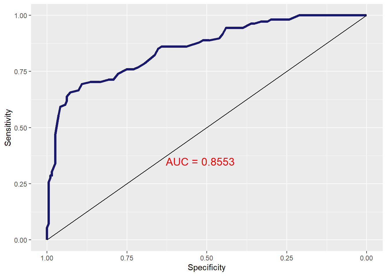

Figure 4.1: ROC Curve for Training Sample

Video Tutorial: Model Fit - ROC Curve

4.7 Gain/Lift Charts and Tables

To get the Gain/Lift charts and tables , use the gainlift() function from the MKT4320BGSU course package.
Usage: OBJ.NAME <- gainlift(MOD, TRAIN, TEST, "POS")
- OBJ.NAME is the name of the object to assign the results to
- MOD is the name of the object with results of the glm() call
- TRAIN is the name of the data frame containing the training sample
- TEST is the name of the data frame containing the test/holdout sample
- "POS" is the level of the factor variable that is the SUCCESS level
This function requires the ggplot2, dplyr, and tidyr packages, which need to be loaded first

This user defined function returns a list of four objects

To use, assign the result to an object name, and then call one of the four objects returned from the function

 # Load necessary packages (if not already loaded)
library(ggplot2)
library(dplyr)
library(tidyr)

# Call the function and assign to object named 'glresults'
glresults <- gainlift(model,  # Name of the glm results object
                      train,  # Name of the training data frame
                      test,   # Name of the testing data frame
                      "Yes")  # Level that represents success/true

OBJ.NAME$gaintable returns the Gain table

glresults$gaintable

# A tibble: 20 × 3
   `% Sample` Holdout Training
        <dbl>   <dbl>    <dbl>
 1       0.05   0.114    0.130
 2       0.1    0.229    0.269
 3       0.15   0.371    0.370
 4       0.2    0.457    0.5  
 5       0.25   0.6      0.602
 6       0.3    0.714    0.667
 7       0.35   0.8      0.704
 8       0.4    0.8      0.731
 9       0.45   0.829    0.769
10       0.5    0.886    0.815
11       0.55   0.914    0.861
12       0.6    0.943    0.870
13       0.65   0.971    0.889
14       0.7    1        0.944
15       0.75   1        0.954
16       0.8    1        0.972
17       0.85   1        0.991
18       0.9    1        1    
19       0.95   1        1    
20       1      1        1

Table 4.8: Gain Table

OBJ.NAME$gainplot returns the Gain plot

glresults$gainplot

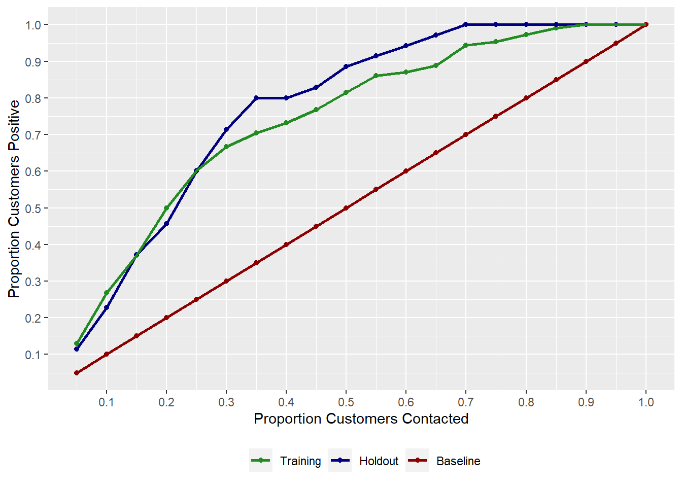
Figure 4.2: Gain Plot

OBJ.NAME$lifttable returns the Lift table

glresults$lifttable

# A tibble: 20 × 3
   `% Sample` Holdout Training
        <dbl>   <dbl>    <dbl>
 1       0.05    2.83     2.60
 2       0.1     2.51     2.69
 3       0.15    2.63     2.48
 4       0.2     2.38     2.51
 5       0.25    2.48     2.42
 6       0.3     2.44     2.23
 7       0.35    2.33     2.02
 8       0.4     2.03     1.83
 9       0.45    1.86     1.71
10       0.5     1.79     1.64
11       0.55    1.68     1.57
12       0.6     1.58     1.46
13       0.65    1.50     1.37
14       0.7     1.43     1.35
15       0.75    1.34     1.28
16       0.8     1.25     1.22
17       0.85    1.18     1.17
18       0.9     1.11     1.11
19       0.95    1.05     1.06
20       1       1        1

Table 4.9: Lift Table

OBJ.NAME$liftplot returns the Lift plot

glresults$liftplot

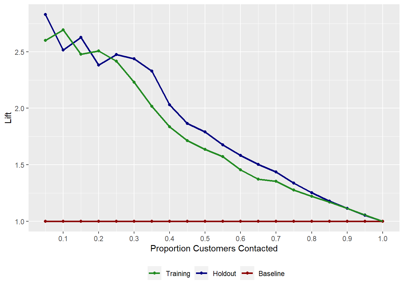
Figure 4.3: Lift Plot

Video Tutorial: Model Performance - Gain and Lift

4.8 Sensitivity/Specificity Plot

To get the Sensitivity/Specificity plot, use the logreg_cut() function from the MKT4320BGSU course package.
Usage: logreg_cut(MOD, DATA, "POS")
- MOD is the name of the object with results of the glm() call
- DATA is the data set for which the plot should be produced (i.e., original, training, or testing)
- "POS" is the level of the factor variable that is the SUCCESS level

This function requires the ggplot2 package, which needs to be loaded first

# Load necessary packages
library(ggplot2)

# Sensitivity/Specificity Plot for Training Sample
logreg_cut(model,  # Name of the results object
          train,   # Use training sample
          "Yes")   # Level of 'buy' that represents success/true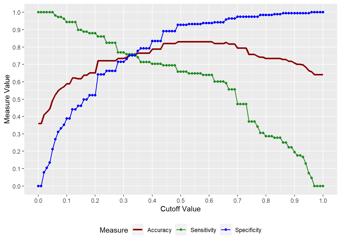

Figure 4.4: Sensitivity/Specificity Plot for Training Sample

Video Tutorial: Logistic Regression - Sensitivity/Specificity Plots

4.9 Margin Plots

Margin plots are done in much the same way as with linear regression margin plots

# Create plot for 'age' and assign to 'p1'
p1 <- mymp(model, "age")$plot

# Create plot for 'gender' and assign to 'p2'
p2 <- mymp(model, "gender")$plot

#Use 'cowplot' to put into single plot
cowplot::plot_grid(p1,p2)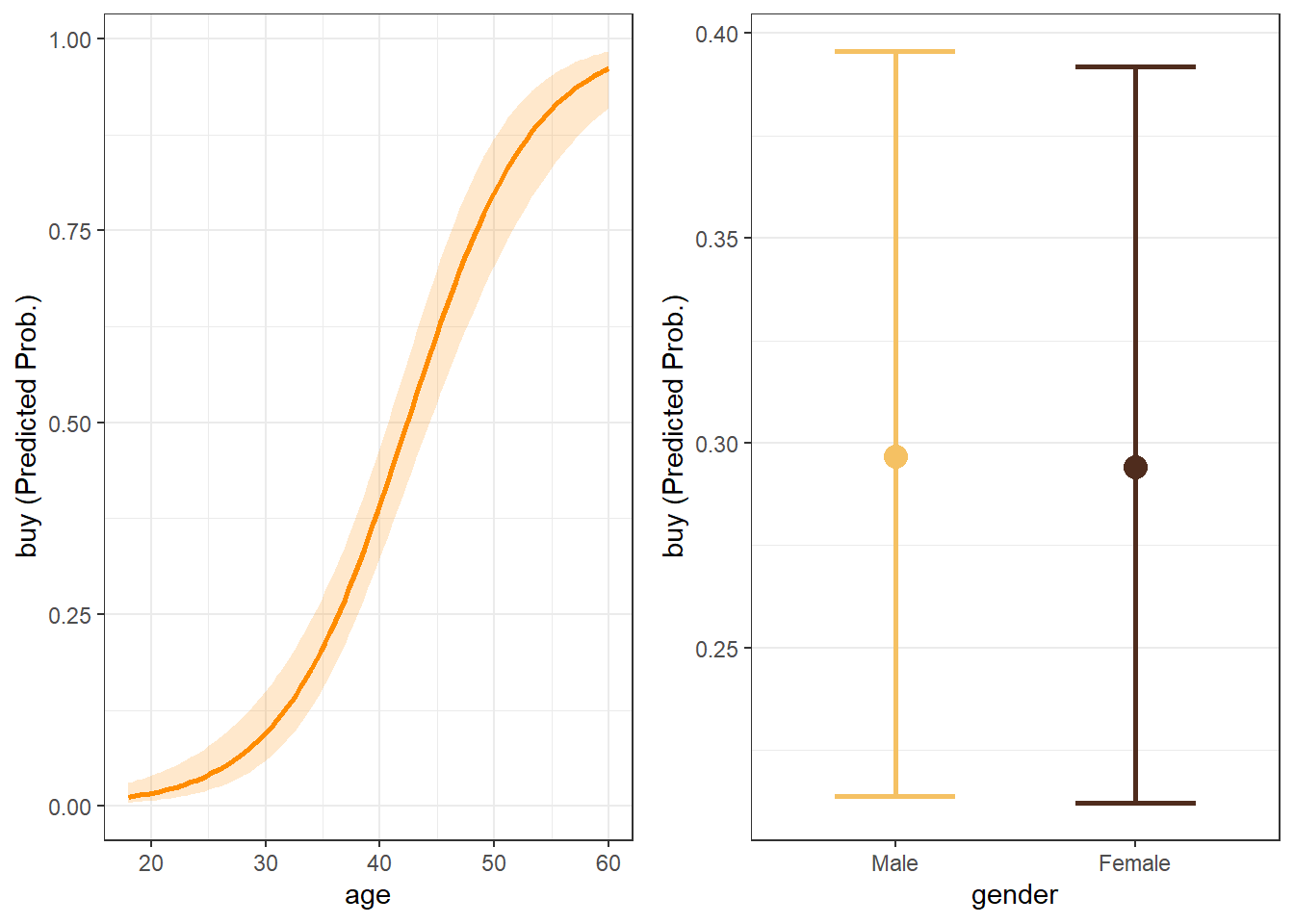

Figure 4.5: Margin plots for variables in model

Video Tutorial: Logistic Regression - Margin Plots