Chapter 5 Cluster Analysis

Sources for this chapter:

• R for Marketing Research ad Analytics, Second Edition (2019). Chris Chapman and Elea McDonnell Feit
  • http://r-marketing.r-forge.r-project.org/index.html

Data for this chapter:

• The ffseg data is used from the MKT4320BGSU course package. Load the package and use the data() function to load the data.

  # Load the course package
  library(MKT4320BGSU)
  # Load the data
  data(ffseg)

5.1 Introduction

Base R is typically sufficient for performing the basics of both hierarchical and k-means cluster analysis, but to get some of the outputs required more easily and more efficiently, I have created some user defined functions. You should download these functions and save them in your working directory.

• clustop provides Duda-Hart and psuedo-\(T^2\) indices for hierarchical agglomerative clustering
• cldescr describes variables based on cluster membership
• myhc produces a dendrogram and cluster sizes and percents for hierarchical agglomerative clustering
• wssplot produces a scree plot for \(k\)-means
• ksize produces cluster size and proportion tables for \(k\)-means
• kcenters produces cluster center table and plot from \(k\)-means

5.2 Preparation

• For both hierarchical agglomerative and k-means clustering, we usually prepare our data for clustering
  • In other words, choose which variable to use for clustering
  • Package dplyr is usually the best tool for this

library(dplyr)
# Store variables selected using dplyr to 'segvar'
clvar <- ffseg %>%   
    select(quality, price, healthy, variety, speed)

* To standardize the clustering variables, use the `scale` function
    * Usage: `scale(data)`
    * To store as a data frame, wrap the command in `data.frame()`

# Standardize 'clvar' df and store as 'sc.clvar'
sc.clvar <- data.frame(scale(clvar))  

Video Tutorial: Cluster Analysis Introduction and Preparation

5.3 Hierarchical Agglomerative Clustering

5.3.1 Base R

• In Base R, hierarchical cluster analysis is done in multiple steps,
  1. Use the dist() function to create a similarity/dissimilarity matrix
  2. Use the hclust() function to perform hierarchical cluster analysis on the matrix from (1)
  3. Determine how many clusters are desired using a dendrogram and/or the stopping indices from package NbClust

5.3.1.1 Creating the similarity/dissimilarity matrix

• Usage: dist(data, method="") where:
  • data is the (scaled) cluster variable data
  • method="" indicates the distance measure:
    • method="euclidean" provides Euclidean distance
    • method="maximum" provides Maximum distance
    • method="manhattan" provides Absolute distance
    • method="binary" provides a distance measure for a set of binary-only variables
    • NOTE: other choices exist, but for MKT 4320, our focus is on these four

# Create the similarity/dissimilarity matrix and save as object 'dist'
dist <- dist(sc.clvar,   # Scaled data from earlier
             method="euclidean")    # Euclidean distance measure

Video Tutorial: HCA in Base R - Creating Similarity Matrix

5.3.1.2 Perform hierarchical clustering

• Usage: hclust(d, method="") where:
  • d is the similarity/dissimilarity matrix
  • method="" indicates the linkage method:
    • method="single" provides Single linkage
    • method="complete" provides Complete linkage
    • method="average" provides Average linkage
    • method="ward.D" provides Ward’s linkage
    • NOTE: other choices exist, but for MKT 4320, our focus is on these four

# Preform hierarchical clustering and save as object 'hc'
hc <- hclust(dist,  # similarity/dissimilarity matrix from earlier
             method="ward.D")   # Ward's linkage method

# NOTE: The similarity/dissimilarity matrix can be done within the call
#       to 'hclust'
hc1 <- hclust(dist(sc.clvar, method="euclidean"), method="ward.D")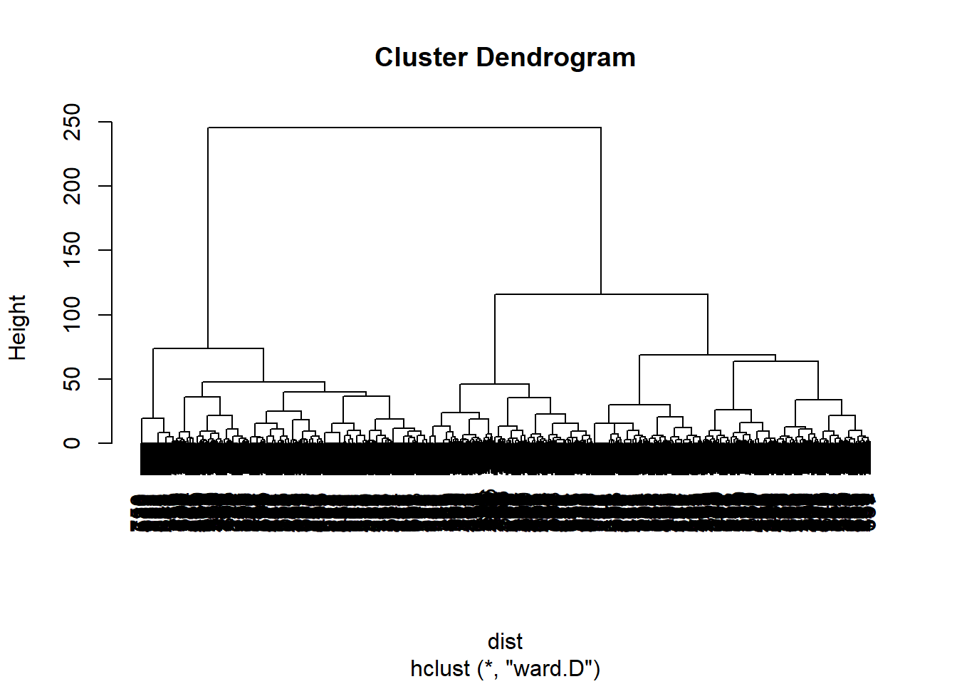

5.3.1.3 Create a dendrogram

• Usage: plot(x) where:
  • x is a hierarchical clustering object

# Create dendrogram of object hc
plot(hc)

Video Tutorial: HCA in Base R - Running the Analysis

5.3.1.4 Stopping indices

• To get the Duda-Hart index, and the pseudo-\(T^2\), the NbClust package is used
  • This package is not available in BGSU’s Virtual Computing Lab
• Usage: NbClust(data, distance="", method="", min.nc=, max.nc=, index="")$All.index where:
  • data is the (scaled) cluster variable data
  • distance="" indicates the distance measure using the same options from the dist function above
  • method="" indicates the linkage method using the same options from the hclust option above
  • min.nc= and max.nc= indicate the minimum and maximum number of clusters to examine
  • index="" indicates what measure is wanted:
    • index="duda" uses the Duda-Hart index
    • index="pseudot2 uses the pseudo-\(T^2\) index
  • $All.index requests only the index values be returned

# After installing package for the first time, load the 'NbClust' package
library(NbClust)
# Get Duda-Hart Index
NbClust(sc.clvar,   # Scaled cluster variable data from earlier
        distance="euclidean",   # Euclidean distance measure
        method="ward.D",   # Ward's linkage
        min.nc=1,   # Show between 1 and...
        max.nc=10,  # ... 10 clusters
        index="duda")$All.index   # Request Duda-Hart index

     1      2      3      4      5      6      7      8      9     10 
0.7974 0.8367 0.8435 0.8490 0.7448 0.8628 0.8222 0.8206 0.6950 0.6470 

# Get pseudo-T2
NbClust(sc.clvar, distance="euclidean", method="ward.D",
        min.nc=1, max.nc=10, index="pseudot2")$All.index

       1        2        3        4        5        6        7        8 
190.5756  88.3818  54.7376  50.5151  58.5770  41.3604  36.1142  40.0002 
       9       10 
 46.9583  40.9146 

Video Tutorial: HCA in Base R - Stopping Indices using NbClust

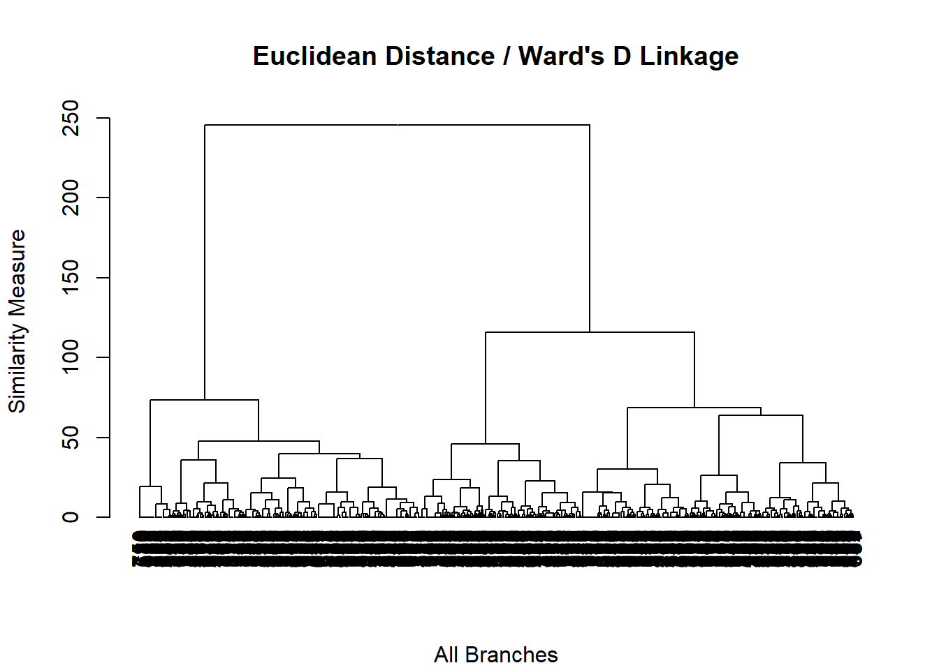
5.3.2 User Defined Functions

• The myhc.R user defined function can produce the results with one or two passes of the function
  • Requires the following packages:
    • dendextend
    • dplyr
    • NbClust
• The results should be saved to an object
• Usage: myhc(data, dist="", method="", cuts, clustop="") where:
  • data is the (scaled) cluster variable data
  • dist="" indicates the distance measure:
    • dist="euc" provides Euclidean distance
    • dist="euc2" provides Euclidean Squared distance
    • dist="max" provides Maximum distance
    • dist="abs" provides Absolute distance
    • dist="bin" provides a distance measure for a set of binary-only variables
  • method="" indicates the linkage method:
    • method="single" provides Single linkage
    • method="complete" provides Complete linkage
    • method="average" provides Average linkage
    • method="ward" provides Ward’s linkage
  • cuts indicates how many clusters (optional):
    • Examples: cuts=3; cuts=c(2,4,5)
  • clustop="" indicates if stopping indices are wanted
    • clustop="Y" if indices are wanted
    • clustop="N" if indices are not wanted
• Objects returned:
  • If cuts are provided:
    • Dendrogram of the top \(n\) branches, where \(n\) is the highest number of clusters provided by cuts
    • Table of cluster sizes ($kcount)
    • Table of cluster size percentages ($kperc)
    • hclust object ($hc)
    • Stopping indices for 1 to 10 clusters, if requested ($stop)
  • If cuts are not provided:
    • Dendrogram with all branches
    • Stopping indices for 1 to 10 clusters, if requested ($stop)

Video Tutorial: HCA Using myhc.R (Part 1)

• Examples:

  • No cuts with stopping indices

  # Both myhc.R and clustop.R need to be "sourced"
  eg1 <- myhc(sc.clvar, "euc", "ward", clustop="Y")

  

  # Dendrogram will get produced automatically
  # Call eg1$stop to get table of stopping indices
  eg1$stop

     Num.Clusters Duda.Hart pseudo.t.2
  1             1    0.7974   190.5756
  2             2    0.8367    88.3818
  3             3    0.8435    54.7376
  4             4    0.8490    50.5151
  5             5    0.7448    58.5770
  6             6    0.8628    41.3604
  7             7    0.8222    36.1142
  8             8    0.8206    40.0002
  9             9    0.6950    46.9583
  10           10    0.6470    40.9146

  • One cut without stopping indices

  eg2 <- myhc(sc.clvar, "max", "ward", cuts=5, clustop="N")

  

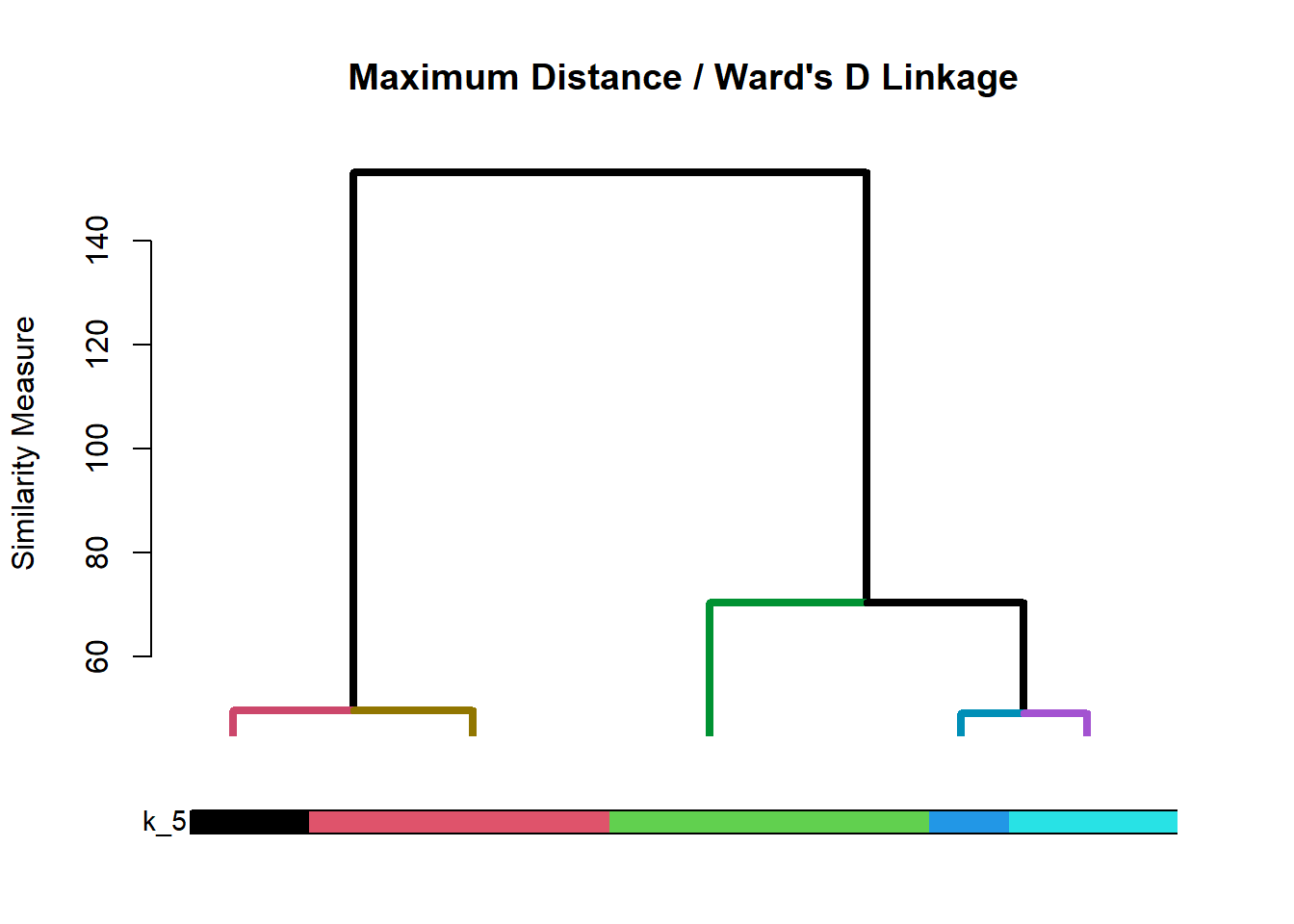
  # Dendrogram will get produced automatically
  # call eg2$kcount and eg2$kperc to get cluster sizes
  eg2$kcount

    Cluster k_5_Count
  1       1       244
  2       2       229
  3       3       127
  4       4        91
  5       5        61

  eg2$kperc

    Cluster k_5_Percent
  1       1       32.45
  2       2       30.45
  3       3       16.89
  4       4       12.10
  5       5        8.11

  • Multiple cuts without stopping indices

  eg3 <- myhc(sc.clvar, "abs", "ward", cuts=c(2,3,4,6), clustop="N")

  

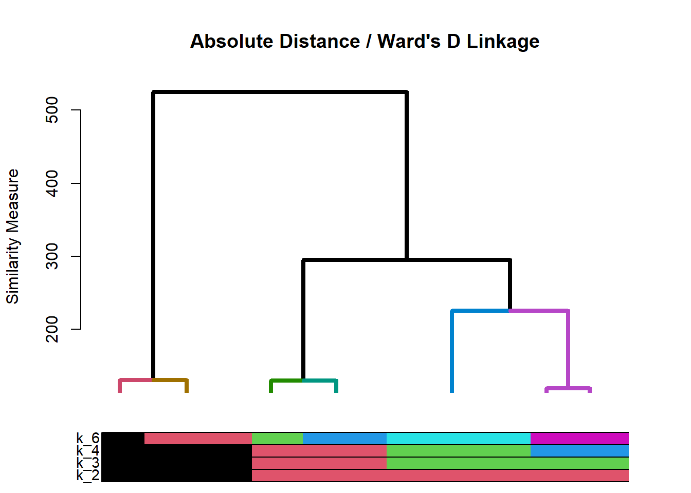
  # Dendrogram will get produced automatically
  # call eg3$kcount and eg3$kperc to get cluster sizes
  eg3$kcount

    Cluster k_2_Count k_3_Count k_4_Count k_6_Count
  1       1       537       344       215       205
  2       2       215       215       205       153
  3       3        NA       193       193       139
  4       4        NA        NA       139       120
  5       5        NA        NA        NA        73
  6       6        NA        NA        NA        62

  eg3$kperc

    Cluster k_2_Percent k_3_Percent k_4_Percent k_6_Percent
  1       1       71.41       45.74       28.59       27.26
  2       2       28.59       28.59       27.26       20.35
  3       3          NA       25.66       25.66       18.48
  4       4          NA          NA       18.48       15.96
  5       5          NA          NA          NA        9.71
  6       6          NA          NA          NA        8.24

Video Tutorial: HCA with myhc.R (Part 2) Video Tutorial: HCA with myhc.R (Part 3)

5.3.3 Cluster membership

• Use the cutree() function to get cluster membership for the specified number of clusters
• Usage: cutree(tree, k=) where:
  • tree is an hclust object from Base R methods or from myhc function
  • k= is the number of clusters to retrieve
• Assign cluster membership to original data, cluster variables, or both

# Create new variables in original data based on cluster membership
# Need to use 'as.factor()' to classify variable as factor
ffseg$K3 <- as.factor(cutree(hc,  # 'hclust' object from Base R earlier
                             k=3))   # Number of clusters to retrieve
ffseg$K4 <- as.factor(cutree(eg3$hc, # 'hclust' object from call to 'myhc' earlier
                             k=4))   # Number of clusters to retrieve

# Create new data frame of scaled clustering variables
# with cluster membership appended
# 'cbind' stands for column bind
sc.cldesc <- cbind(sc.clvar,  # Scaled cluster variables
                   K3=as.factor(cutree(hc, k=3)))  # Cluster membership variable

Video Tutorial: Assigning Cluster Membership after HCA with cutree(https://youtu.be/86uktpw0jSQ)

5.4 k-Means Clustering

5.4.1 Base R

• \(k\)-Means clustering is done mostly in Base R, but there is a couple user defined functions to help
• Process:
  • Run wssplot.R user defined function to get a scree plot
  • Based on scree plot, use ksize() user defined function to examine the cluster sizes for several solutions
  • Run kmeans() for desired solution
  • Assign cluster membership for desired number of clusters to original data, cluster variables, or both

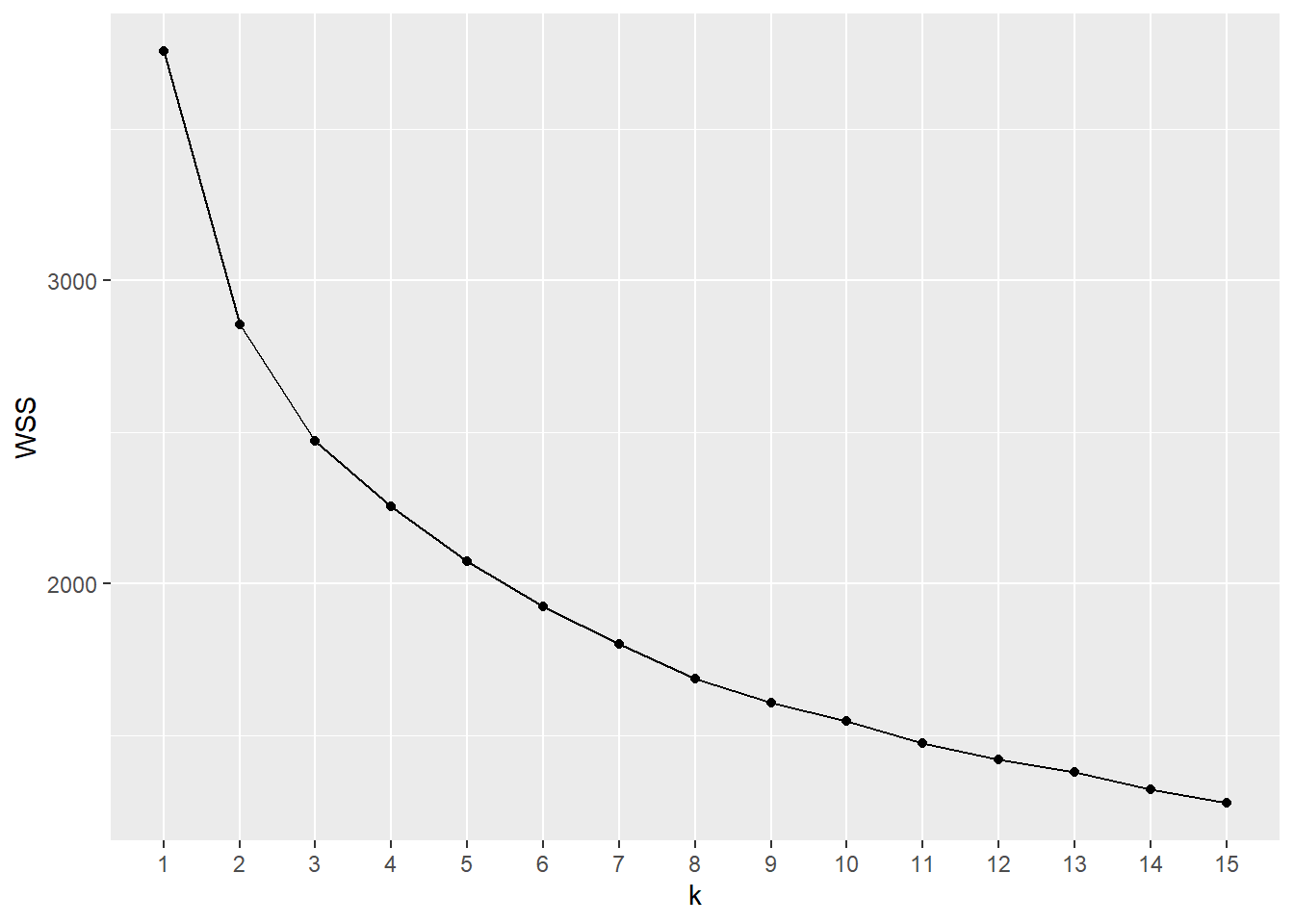
5.4.1.1 Scree plot

• The wssplot.R user defined function produces a scree plot for 1 to \(n\) clusters
  • Requires the ggplot2 package
• Usage: wssplot(data, nc=, seed=) where:
  • data is the (scaled) cluster variable data
  • nc= takes an integer value and is the maximum number of clusters to plot; default is 15
  • seed= is a random number seed for reproducible results; default is 4320

wssplot(sc.clvar)  # Produces scree plot with default 15 clusters and 4320 seed

5.4.1.2 Cluster sizes

• The ksize.R user defined function produces a count and proportion tables for the selected \(k\) solutions
• The results should be saved to an object
• Usage: ksize(data, centers=, nstart=, seed=) where:
  • data is the (scaled) cluster variable data
  • centers= takes one or more integers for the \(k\) cluster solutions to be examined
  • nstart= takes an integer value for the number of random starting points to try; default is 25
  • seed= is a random number seed for reproducible results; default is 4320
• Objects returned:
  • Table of cluster sizes ($kcount)
  • Table of cluster size percentages ($kperc)

ks <- ksize(sc.clvar,   # Scaled cluster variables from earlier
            centers=c(3,4,5),   # Request for 3, 4, and 5 cluster solutions
            nstart=25,  # Request 25 random starting sets
            seed=4320)  # Set seed to 4320 for reproducible results
ks$kcount   # Cluster sizes

  Num_Clusters k_3_Count k_4_Count k_5_Count
1            1       308       211       205
2            2       238       191       167
3            3       206       187       150
4            4        NA       163       124
5            5        NA        NA       106

ks$kperc     # Cluster percentages

  Num_Clusters k_3_Percent k_4_Percent k_5_Percent
1            1       40.96       28.06       27.26
2            2       31.65       25.40       22.21
3            3       27.39       24.87       19.95
4            4          NA       21.68       16.49
5            5          NA          NA       14.10

Video Tutorial: k-Means Cluster Analysis - How Many Clusters?

5.4.1.3 kmeans function

• Usage: kmeans(data, centers=, nstart=) where:
  • data is the (scaled) cluster variable data
  • centers= takes an integer value for the number of clusters desired
  • nstart= takes an integer value for the number of random starting points to try
• Results should be assigned to an object
• NOTE 1: For reproducible results, set.seed() should be run immediately before running kmeans()
• NOTE 2: nstart= should be same value as above
• Use the saved $cluster object to assign cluster membership

set.seed(4320)  # Set random number seed
# Run kmeans() for 4 clusters and assign to object k3
k4 <- kmeans(sc.clvar,   # Scaled cluster variables from earlier
             centers=4,  # Request 3-cluster solution
             nstart=25)  # Request 25 random starting sets
ffseg$KM4 <- as.factor(k4$cluster)

Video Tutorial: Using the kmeans() Function

5.5 Describing clusters

5.5.1 cldescr.R

• The cldescr.R user defined function can be used to describe the clusters on both cluster variables and other variables that may be in the dataset
• The results should be assigned to an object
• Usage: cldescr(data, var="", vtype=c("F", "C"), cvar="" where:
  • data is the original data or (scaled) cluster variable data with cluster membership attached
  • var="" contains the name of the variable to examine by cluster membership
  • vtype="" takes “F” if var is a factor variable or “C” if var is a continuous variable
  • cvar="" contains the name of the cluster membership variable
• If vtype="F" with more than two levels, the factor variable is split into dummy variables (1=True, 0=False) for each level of the factor
• If vtype="F" with only two levels, the only the first level of the factor variable is shown as a dummy variable (1=True, 0=False)
• If vtype="C" a list (using c()) of variables can be provided
• Objects returned
  • Table of means ($means)
    • If vtype="F", one column per level of factor
  • Table of ANOVA p-values ($aovp)
  • Table(s) of Tukey HSD multiple comparisons for any variables where the ANOVA p-value\(<0.1\) (tukey)

Video Tutorial: Describing clusers using cldescr.R (Part 1)

5.5.1.1 Examples

• Describing hierarchical clustering using clustering variables

hc.cv <- cldescr(sc.cldesc,    # Scaled cluster variables w/ cluster membership
                 var=c("quality", "price", "healthy", # List of cluster variables
                   "variety", "speed"),
                 vtype="C",  # All variables are continuous
                 cvar="K3")  # Cluster membership variable
hc.cv$means

  Cluster quality   price healthy variety   speed
1       1  0.7033  0.0515  0.7903  0.5729  0.3159
2       2 -0.5419  0.5722 -0.5865 -0.3641  0.0258
3       3 -0.3189 -1.0589 -0.3964 -0.3907 -0.5989

hc.cv$aovp

  Variable p.value
1  quality       0
2    price       0
3  healthy       0
4  variety       0
5    speed       0

# hc.cv$tukey   # NOT SHOWN BECAUSE USUALLY ALL SIGNIFICANTLY DIFFERENT 

• Describing hierarchical clustering or \(k\)-means using non-clustering continuous variables done the same as previous example
• Describing hierarchical clustering or \(k\)-means using non-clustering factor variables

#  Factor variable 'live' on k-means solution
km.fv <- cldescr(ffseg, var="live", vtype="F", cvar="KM4")
km.fv$means

  Cluster Commuter Off.Campus On.Campus
1       1   0.1123     0.4545    0.4332
2       2   0.0613     0.4417    0.4969
3       3   0.1623     0.3665    0.4712
4       4   0.0758     0.4929    0.4313

km.fv$aovp

    Variable p.value
1   Commuter  0.0069
2 Off.Campus  0.0805
3  On.Campus  0.5349

km.fv$tukey

$Commuter
       diff  p adj
2-1 -0.0509 0.3977
3-1  0.0500 0.3776
4-1 -0.0365 0.6286
3-2  0.1010 0.0101
4-2  0.0145 0.9681
4-3 -0.0865 0.0229

$Off.Campus
       diff  p adj
2-1 -0.0128 0.9950
3-1 -0.0881 0.3101
4-1  0.0383 0.8677
3-2 -0.0752 0.4848
4-2  0.0512 0.7550
4-3  0.1264 0.0528

#  Factor variable 'gender' on hierarchcial clustering solution
hc.fv <- cldescr(ffseg, var="gender", vtype="F", cvar="K3")
hc.fv$means

  Cluster Female
1       1 0.8182
2       2 0.6783
3       3 0.5917

hc.fv$aovp

  Variable p.value
1   Female       0

hc.fv$tukey

       diff  p adj
2-1 -0.1399 0.0004
3-1 -0.2265 0.0000
3-2 -0.0866 0.1100

Video Tutorial: Describing clusers using cldescr.R (Part 2) Video Tutorial: Describing clusers using cldescr.R (Part 3)

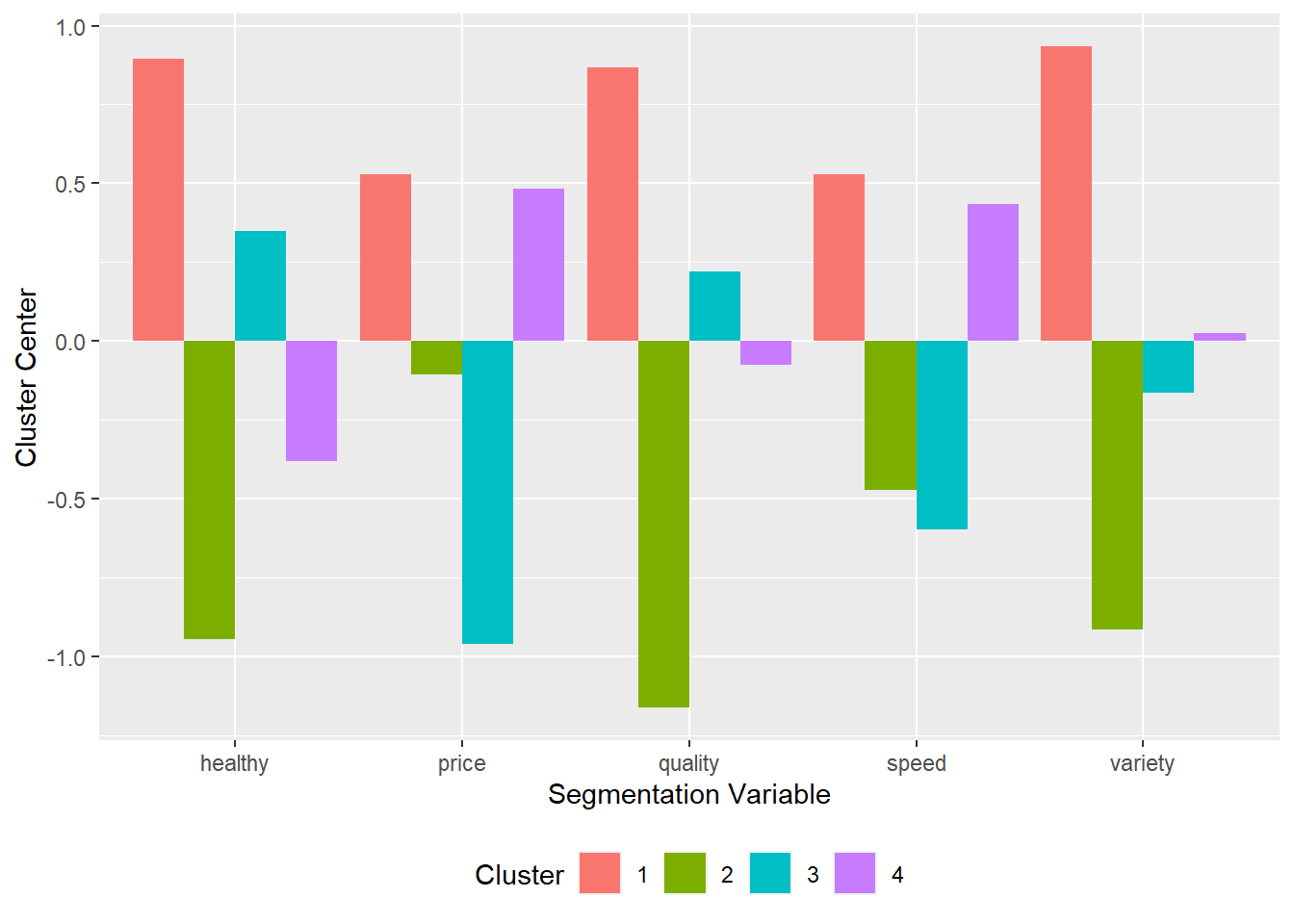
5.5.2 kcenters.R

• For \(k\)-Means, the kcenters.R user defined function can be used to describe the cluster centers
  • Requires ggplot2 package
• The results should be assigned to an object
• Usage: kcenters(kobject) where:
  • kobject is the name of a saved \(k\)-means object
• Objects returned
  • Table of means ($table)
  • ggplot object ($plot)
• Describing \(k\)-means clustering using cluster centers

km.cent <- kcenters(k4)
km.cent$table

      quality      price    healthy     variety      speed Cluster
1  0.86830982  0.5282993  0.8952494  0.93322588  0.5295407       1
2 -1.15981355 -0.1062743 -0.9446355 -0.91358591 -0.4716217       2
3  0.22194885 -0.9606064  0.3494969 -0.16288116 -0.5958141       3
4 -0.07448606  0.4834435 -0.3800472  0.02612117  0.4343635       4

km.cent$plot

Video Tutorial: Describing clusers using kcenters.R