Chapter 1 R Basics

Sources for this chapter:

• R for Marketing Research ad Analytics, Second Edition (2019). Chris Chapman and Elea McDonnell Feit
  • http://r-marketing.r-forge.r-project.org/index.html

1.1 Introduction

1.1.1 What is R?

• R is a programming language
• R is not a statistics program
  • Much different than SPSS, MiniTab, Stata, etc.
  • Does not use a point-and-click interface

1.1.2 Why R?

• Emerging techniques usually available in R quickly
• Default educational platform for statistics programs (and spreading to other disciplines)
• Large and diverse set of analytic tools
• Powerful plotting options
• Large community of helpful users
• R skills are in high demand

And

• R is free

1.1.3 Why NOT R?

• Steep learning curve
• Requires programming

1.1.4 What is RStudio?

• RStudio IDE is an integrated development environment that makes working with R more user friendly
• Not required to use R, but provides a better interface and environment of writing code, editing code, and creating documents.
• Complete separate software

And

• RStudio is free

1.1.5 Getting Started

1.1.5.1 Option 1: Install on your Machine

1. Install “R base” from the Comprehensive R Archive Network (CRAN)
   • https://cran.r-project.org/
2. Install RStudio
   • https://posit.co/download/rstudio-desktop/#download

1.1.5.2 Option 2: Use BGSU’s Virtual Computing Lab pilot

• See course website for link

1.1.5.3 Option 3: Use a computer in an on-campus computer lab

• All computer in on-campus computer labs should have R and RStudio installed

1.1.6 Navigating RStudio

As you can see in Figure 1.1, RStudio is typically divided in 4 quadrants.

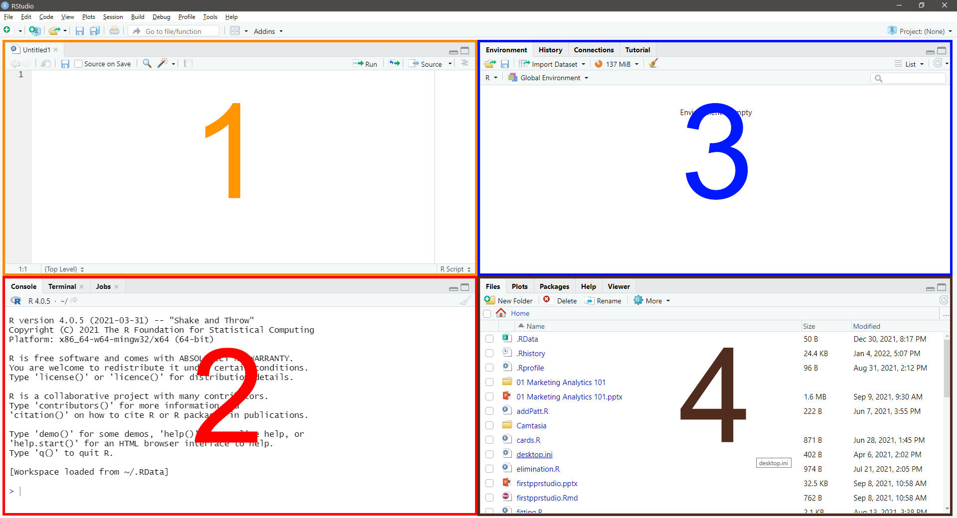
Figure 1.1: RStudio Layout

1.1.6.1 Quadrant 1

The upper-left corner is the source pane. This pane is where the majority of your programming or coding will take place. When working in this pane, the code does not run unless you tell it to run. In addition, the code can be saved to prevent work from being lost.

1.1.6.2 Quadrant 2

The lower-left corner is the console pane. While it contains several tabs, generally the Console tab is the only one used. The console is where R actually evaluates the code. If you run code from the a source pane window, the code will automatically be put into the console pane and evaluated. You can also type code directly into the console pane and receive immediate results. Depending on the code, the results will appear directly in the console or in a tab Quadrant 4. The “>” symbol shows that the console is ready for input.

1.1.6.3 Quadrant 3

The upper-right corner also contains several tabs, but the Environment and History tabs are the ones used most often.

• The Environment tab lists all data objects that have been defined in the current session.
• The History tab is an archive of all commands run in the current session.

1.1.6.4 Quadrant 4

The bottom-right corner also contains several tabs, all of which are used at different times.

• The Files tab lists all files in the current directory.
• The Plots tab shows visualizations created during the current session.
• The Packages tab shows all packages installed as well as which packages are currently loaded.
• The Help tab contains the help menu.
• The Viewer tab contains output from code if the code directs it to be displayed there.

1.2 R Language

1.2.1 Basics of R Commands

• R is case sensitive
• When using the console, use the keyboard  ↑  and  ↓  arrow keys to easily cycle through previous commands typed.
• When using the text editor (i.e., a script file) in the source pane, use the Ctrl+Enter keyboard shortcut to submit a line of code directly to the console.
  • The entire line does not need to be highlighted; the cursor needs to be anywhere on the line to be submitted.
• When using the text editor/script file, the “#” symbol signifies a comment
  • Everything after is ignored
  • It can be on the same line:

  x <- 100   # Assign 100 to x

  • It can be on separate lines:

  # Assign 100 to x
  x <- 100

1.2.2 Operators

Mathematical and logical operators are used frequently.

Table 1.1: R Operators

Description	Operator
Mathematical
addition	\(+\)
subtraction	\(-\)
multiplication	\(*\)
division	\(/\)
exponentiation	^ or \(**\)
Logical
less than	<
less than or equal to	<=
greater than	>
greater than or equal to	>=
exactly equal to	==
not equal to	!=
Not x	!x
x OR y	x|y
x AND y	x&y
test if X is TRUE	isTRUE(x)

1.3 Packages

Packages are collections of functions that have been written to expand the functionality of R. Packages are not automatically included, and if a command is given that is not part of a package installed and loaded, R will give an error message. Therefore, the package must first be installed, and then loaded.

1.3.1 Installing Packages

• Installing packages is performed with the install.packages("")function, where the name of the package is inside the quotation marks

• Two packages that used quite often in this course are ggplot2 and dplyr

  install.packages("ggplot2")
  install.packages("dplyr")

• NOTE 1: Packages only need to be installed on your machine once

• NOTE 2: If using BGSU’s Virtual Computing Lab, new packages cannot be installed, but the version in the virtual environment has most of the most common packages pre-installed

1.3.2 Loading Packages

• Once a package is installed, it has to be loaded with the library() function, where the name of the package is in the parentheses, in order to be used

  library(ggplot2)
  library(dplyr)

• NOTE 1: It is not uncommon to see a variety of messages when loading a package

• NOTE 2: Packages need to be loaded every time you start a new R session

1.4 Getting Help

• R has built in help to assist with understanding different functions

• To access the help, type ? FUNCTION in the console, and the help page for that function will show up in the lower-right pane under the help tab

  ? mean

1.5 Basic Object Types (and Other Important Stuff)

• Objects in R include variables, data sets, and functions

• The assignment operator <- assigns a value to a named object

  x <- 100     # Assign value 100 to object 'x'
  x            # Display object 'x'

  [1] 100

  NOTE: In RStudio console or script file, Alt+- will automatically paste the assignment operator

• As stated before, object names are case sensitive

  x <- 100     # Assign value 100 to object 'x'
  X            # Display object 'X'

  Error in eval(expr, envir, enclos): object 'X' not found

• The print command can also be used to print objects

  print(x)

  [1] 100

Video Tutorial: Assignment Operator

1.5.1 Vectors

• Vectors can be created many ways and take many data types

• One method is to using the c() function, which concatenates individual items

  x.Num <- c(1, 3.14, 5.49, 10, 20)
  x.Num

  [1]  1.00  3.14  5.49 10.00 20.00

  x.Log <- c(TRUE, FALSE, TRUE, TRUE, FALSE)
  x.Log

  [1]  TRUE FALSE  TRUE  TRUE FALSE

  x.Char <- c("fr", "fr", "jr", "so", "sr")
  x.Char

  [1] "fr" "fr" "jr" "so" "sr"

• The class of the vector can be checked with the class() function

  # Concatenate class functions and print together
  print(c(class(x.Num), class(x.Log), class(x.Char)))

  [1] "numeric"   "logical"   "character"

Video Tutorial: Vectors - Part 1

• Vectors can only hold a single class/type of value

  • When multiple classes are included, the values are coerced to the most general type

  x.Mix <- c(1, FALSE, 3.5, "Hello!")
  x.Mix

  [1] "1"      "FALSE"  "3.5"    "Hello!"

  class(x.Mix)

  [1] "character"

• The c() function can be used to add to existing vectors, or combine vectors

  • Type coercion will be applied as needed

  x2 <- c(x.Num, 25, 50)
  x.Num

  [1]  1.00  3.14  5.49 10.00 20.00

  x2

  [1]  1.00  3.14  5.49 10.00 20.00 25.00 50.00

  x3 <- c(x2, "Hello")
  x3

  [1] "1"     "3.14"  "5.49"  "10"    "20"    "25"    "50"    "Hello"

• Math can be applied directly to vectors

  x.Num

  [1]  1.00  3.14  5.49 10.00 20.00

  x.Num + 100

  [1] 101.00 103.14 105.49 110.00 120.00

  x.Num * pi

  [1]  3.141593  9.864601 17.247344 31.415927 62.831853

• The length() function provides the length of a vector

  length(x.Num)

  [1] 5

  length(x.Char)

  [1] 5

• The str() function provide the structure of an object

  • Class, Length, and Value

  str(x.Num)

   num [1:5] 1 3.14 5.49 10 20

  str(x.Char)

   chr [1:5] "fr" "fr" "jr" "so" "sr"

Video Tutorial: Vectors - Part 2

1.5.2 Indexing

• Indexing is used to obtain particular elements of a data structure

• Vectors are indexed with square brackets, []

  # Obtain the third element of the 'x.Num' vector
  x.Num[3]

  [1] 5.49

• Items can be excluded with negative indexing

  # Obtain all elements except the third element of the 'x.Num' vector
  x.Num[-3]

  [1]  1.00  3.14 10.00 20.00

• Indexing also works with logical operators

  # Obtain all elements in 'x.Num' greater than 5
  x.Num[x.Num > 5]

  [1]  5.49 10.00 20.00

Video Tutorial: Indexing

1.5.3 Sequencing

• Vectors can also be created using sequencing

• Integer sequencing is done with #:# coding

  x.Seq <- 1:10
  x.Seq

   [1]  1  2  3  4  5  6  7  8  9 10

• Sequences can also be used in indexing

  # Obtain the second through fourth element of the 'x.Num' vector
  x.Num[2:4]

  [1]  3.14  5.49 10.00

• Complex sequencing can be done using the seq() function

  x.Seq2 <- seq(from=0, to=100, by=20)
  x.Seq2

  [1]   0  20  40  60  80 100

  Note: the from=, to= and by= can be excluded

  x.Seq3 <- seq(0,100,20)
  x.Seq3

  [1]   0  20  40  60  80 100

Video Tutorial: Sequencing

1.5.4 Missing (and Other Interesting) Values

• In R, missing values are assigned a special constant, NA

• NA is not a character value, but a type of its own

• Any math performed on a value of NA becomes NA

  x.Scores <- c(85, 93, NA, NA)
  mean(x.Scores)

  [1] NA

• Many commands contain a option, na.rm=TRUE, to ignore NA data when performing the function

  mean(x.Scores, na.rm=TRUE)

  [1] 89

• NA values can also be removed before performing the function using the na.omit() function

  mean(na.omit(x.Scores))

  [1] 89

• R also has special types for infinity, Inf, and undefined numbers (i.e., “not a number”), NaN

  • To see this in action, take the natural log, log(), of certain numbers

  log(-1)

  [1] NaN

  log(0)

  [1] -Inf

  Notice that R provides a warning when the NaN is found

1.5.5 Factors

• Character data can be converted into nominal factors using the as.factors() function

• Each unique character value will be a level of the factor

  • Behind the scenes, R stores the values as integers, with a separate list of labels

• When the data type is set as a factor, R knows how to handle it appropriately in the model

• The levels can be accessed with the levels() function

  x.Class <- as.factor(x.Char)
  str(x.Class)

   Factor w/ 4 levels "fr","jr","so",..: 1 1 2 3 4

  levels(x.Class)

  [1] "fr" "jr" "so" "sr"

1.6 Data Frames

Data frames are an object type that deserve special attention

1.6.1 Overview

• Most common way to handle data sets in R
• Provide data to statistical functions
• Think of it like a spreadsheet, or a rectangular object where:
  • Columns are varying data types (i.e., variables)
  • Rows are values in each column (i.e, observations)

1.6.2 Creating a data frame

• Can construct a data frame with the data.frame() function

  • Takes as input a set of vectors of the same length

  x.df <- data.frame(x.Num, x.Log, x.Char)
  x.df

    x.Num x.Log x.Char
  1  1.00  TRUE     fr
  2  3.14 FALSE     fr
  3  5.49  TRUE     jr
  4 10.00  TRUE     so
  5 20.00 FALSE     sr

  • Note that the column names are inherited from the contributing vector

• Elements can be indexed using [ROW, COLUMN] notation

  # Obtain the first element of the third row of data frame 'x.df'
  x.df[3,1]

  [1] 5.49

  # Obtain the third element of the second row of data frame 'x.df'
  x.df[2,3]

  [1] "fr"

Video Tutorial: Data Frames (Part 1)

1.6.2.1 Using vectors in-line

• The vectors can be created in line (i.e., not already created)

• If the vectors are of different length, the shorter vector will be repeated IF the longest vector is divisible by the vector

• If a single value is provided instead of a vector, it is repeated for all rows

  x2.df <- data.frame(var1=seq(10,100,10),
                      var2=c("Yes","No"),
                      var3=1:5,
                      var4=100)
  x2.df

     var1 var2 var3 var4
  1    10  Yes    1  100
  2    20   No    2  100
  3    30  Yes    3  100
  4    40   No    4  100
  5    50  Yes    5  100
  6    60   No    1  100
  7    70  Yes    2  100
  8    80   No    3  100
  9    90  Yes    4  100
  10  100   No    5  100

Video Tutorial: Data Frames (Part 2)

1.6.3 Viewing a Data Frame

There are a few ways to view a data frame

1. Type the data frame name in the console

   x.df

     x.Num x.Log x.Char
   1  1.00  TRUE     fr
   2  3.14 FALSE     fr
   3  5.49  TRUE     jr
   4 10.00  TRUE     so
   5 20.00 FALSE     sr

   • With data frames that have many variables, this is cumbersome
   • With data frames with many rows, a “max.print” setting will kick in and not all rows will be shown

2. To view only a few rows of data, the head(DF, n) function can be used, where DF is the name of the data frame, and n (optional) is the number of rows to view, with 10 as the default
   NOTE: The “Salaries” data frame from the car package is being used as an example

   head(Salaries,5)

         rank discipline yrs.since.phd yrs.service  sex salary
   1     Prof          B            19          18 Male 139750
   2     Prof          B            20          16 Male 173200
   3 AsstProf          B             4           3 Male  79750
   4     Prof          B            45          39 Male 115000
   5     Prof          B            40          41 Male 141500

3. Use the function View() or click on the data frame name in the environment tab to see the data farme in the Source pane See Figure 1.2

   

   Figure 1.2: Viewing a Data Frame in the Source Window

Video Tutorial: Data Frames (Viewing)

1.6.4 Indexing and Sequencing

• Indices can be left blank, which selects all of that dimension

  x.df[2, ]   # Obtain all of row 2

    x.Num x.Log x.Char
  2  3.14 FALSE     fr

  x.df[ ,3]   # Obtain all of column 3

  [1] "fr" "fr" "jr" "so" "sr"

• As with vectors, indexing can be done with sequencing and negative indices to omit rows

  x.df[2:3, ]   # Obtain rows 2 and 3

    x.Num x.Log x.Char
  2  3.14 FALSE     fr
  3  5.49  TRUE     jr

  x.df[ ,-2]    # Exclude column 2

    x.Num x.Char
  1  1.00     fr
  2  3.14     fr
  3  5.49     jr
  4 10.00     so
  5 20.00     sr

• Indexing a data frame returns an object, but the object type depends on the indexing

  • Choosing \(n\) rows and and a single column yields a vector of length \(n\)
  • Choosing multiple columns returns a new data frame
  • Use the str() function to verify the new objects structure

  str(x.df[1, 1])   # 1 row and 1 column = vector of length 1

   num 1

  str(x.df[1:3, 2]) # 3 rows and 1 column = vector of length 3

   logi [1:3] TRUE FALSE TRUE

  str(x.df[1, 1:2]) # 1 row and 2 columns = 1 x 2 data frame

  'data.frame':   1 obs. of  2 variables:
   $ x.Num: num 1
   $ x.Log: logi TRUE

  str(x.df[1:4, c(1, 3)])  #4 rows and 2 columns = 4 x 2 data frame

  'data.frame':   4 obs. of  2 variables:
   $ x.Num : num  1 3.14 5.49 10
   $ x.Char: chr  "fr" "fr" "jr" "so"

• Data frames can also be indexed using column names after the $ character

  x.df$x.Char

  [1] "fr" "fr" "jr" "so" "sr"

Video Tutorial: Data Frames (Indexing & Sequencing)

1.7 Data Transformations

• Analysts and researchers often need to create new variables from existing ones or transform existing variables
• Data transformations can usually be accomplished in more than one way
  • Using base R will be shown first
  • After the dplyr package is introduced, a second way will be shown
• For the transformations shown below, either a new variable will be added to the data frame, or an existing variable will be changed
  • However, it is not always required that the data frame be changed
    • Sometimes, a transformation will be done ‘on the fly’ and used only in an analysis, but the data frame remains the same

1.7.1 Creating New Variables

• Adding a new variable is done using code such as df$new <- SOME FUNCTION, where:
  • df is the name of the data frame
  • new is the name for the new variable
  • SOME FUNCTION is the data transformation to take place

  # Create new variable 'NumSq' that is the square of current variable x.Num
  x.df$NumSq <- x.df$x.Num^2
  x.df

    x.Num x.Log x.Char    NumSq
  1  1.00  TRUE     fr   1.0000
  2  3.14 FALSE     fr   9.8596
  3  5.49  TRUE     jr  30.1401
  4 10.00  TRUE     so 100.0000
  5 20.00 FALSE     sr 400.0000

Video Tutorial: Data Transformations (Introduction)

1.7.2 Recoding (Create New)

• In base R, recoding is usually a multi-step process using indexing

  # Recode 'x.Num' into three factors
  x.df$Grp <- "low"   # Create new variable and set all rows to one level
  x.df$Grp[x.df$x.Num>=3 & x.df$x.Num<10] <- "med"   # Create medium level
  x.df$Grp[x.df$x.Num>10] <- "high"   # Create high level
  x.df$Grp <- as.factor(x.df$Grp)   # Set new variable as factor
  str(x.df)   # See structure of data frame with new variable

  'data.frame':   5 obs. of  5 variables:
   $ x.Num : num  1 3.14 5.49 10 20
   $ x.Log : logi  TRUE FALSE TRUE TRUE FALSE
   $ x.Char: chr  "fr" "fr" "jr" "so" ...
   $ NumSq : num  1 9.86 30.14 100 400
   $ Grp   : Factor w/ 3 levels "high","low","med": 2 3 3 2 1

  Notice the & in the code above. It stands for “and”, which tells R that both conditions must be true

Video Tutorial: Data Transformations (Recoding New Variables) Video Tutorial: Data Transformations (Factor Variables)

1.7.3 Recoding (Change Existing)

• Recoding to change an existing variable is done in a similar manner
  • NOTE: Sometimes we have to first change the variable type, such as when the existing variable is a factor

  # Recode 'Grp' into only two factors
  # Change type to 'character'
  x.df$Grp <- as.character(x.df$Grp)
  # Recode 'low' and 'med' to 'very low'
  x.df$Grp[x.df$Grp=="low" | x.df$Grp=="med"] <- "very low"
  # Change back to factor
  x.df$Grp <- as.factor(x.df$Grp)
  str(x.df)

  'data.frame':   5 obs. of  5 variables:
   $ x.Num : num  1 3.14 5.49 10 20
   $ x.Log : logi  TRUE FALSE TRUE TRUE FALSE
   $ x.Char: chr  "fr" "fr" "jr" "so" ...
   $ NumSq : num  1 9.86 30.14 100 400
   $ Grp   : Factor w/ 2 levels "high","very low": 2 2 2 2 1

  Notice the | in the code above. It stands for “or”, which tells R that either condition can be true.

Video Tutorial: Data Transformations (Recoding Existing Variables)

1.8 R Projects

The best way to manage all of the downloads and assignments for this course is to create an R Project. Follow the following steps to create a new R Project.

1. From within RStudio, select File→New Project…
   See Figure 1.3
   If a Save Current Workspace window pops up, select Don’t Save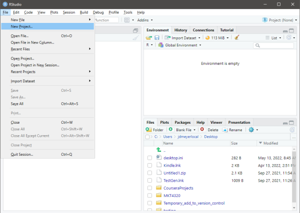
   

   Figure 1.3: Starting a New R Project

2. To create the project in a new directory, select New Directory in the New Project Wizard window, then select New Project. Next, type in the name of the directory in the Directory Name: box (See 1 in Figure 1.4). Next, use the Browse button to select the location of the new directory (See 2 in Figure 1.4). Finally, click on Create Project to create the project (See 3 in Figure 1.4).
   

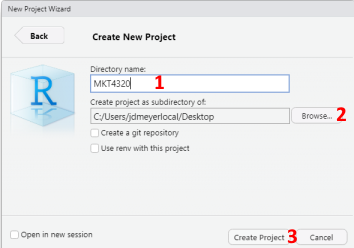
   Figure 1.4: Creating New R Project in New Directory

3. To create the project in an existing directory, select Existing Directory in the New Project Wizard window. Next, use the Browse button to select the location of the existing directory (See 1 in Figure 1.5). Finally, click on Create Project to create the project (See 2 in Figure 1.5).
   

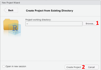
   Figure 1.5: Creating New R Project in Existing Directory

To use the new project each time you work in RStudio for this class, you will need to open the project by using the drop down project menu (See 1 in Figure 1.6) and then selecting the appropriate project (See 2 in Figure 1.6).

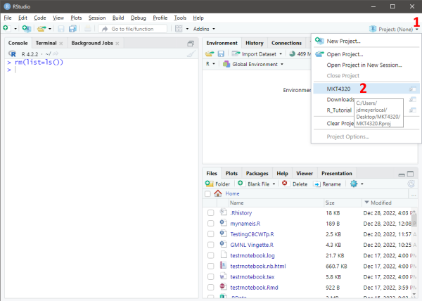
Figure 1.6: Opening an R Project

Video Tutorial: R Projects using New Directory Option

1.9 Loading and Saving Data

In this class, the data will be provided to you as an .Rdata file, which are specific to R and the best way to store (and load) objects. If desired, .Rdata files can contain multiple objects. For example, an .Rdata file could contain two different data frames.

1.9.1 Setting Working Directory

To know where your files are saved to, and to make it easier to load files, it is best to use the R Project discussed above. However, you can also just place all of your files for the course in the same working directory.

• Use the getwd() function to see your current working directory

  getwd()

  [1] "C:/Users/jdmeyer/Documents"

• Set the working directory in one of three ways:

  1. Use the setwd() function:
     setwd("C:/Users/jdmeyer/Doc/RFiles/RTutorial")
     NOTE: Forward slashes (as shown above) are used in place of backward slashes for directory paths
  2. Use the menus in RStudio
     Session→Set Working Directory→Choose Directory
     See Figure 1.7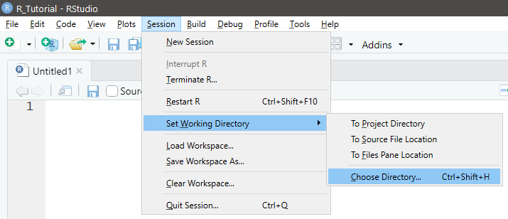
     

     Figure 1.7: Set Working Direcory using Menus

  3. Use the Files tab in the lower-right corner in RStudio
     See Figure 1.8
     

     Figure 1.8: Set Working Direcory using Files Tab

1.9.2 Loading .Rdata

• Use the load("FILE LOCATION/NAME") function to load and .Rdata file
  • Suppose the data set used in Topic 1 (airlinesat.rdata) is in a subdirectory of the working directory called Data

  load("Data/airlinesat.rdata")

  See 1.9 for a visual example
  

  Figure 1.9: Loading Data

1.9.3 Saving .Rdata

• Use the save(OBJECT, file="SAVENAME") function, where:
  • OBJECT is one or more objects in the current environment separated by commas
  • SAVENAME is the name of the file the objects will be saved to.

  save(x.df, file="xdf.rdata")

1.10 User Defined Functions

Often, a series of commands is repeated over and over, or there is not an easy, built-in function in R to provide a needed result. In these case, R makes it relatively easy to create your own functions

1.10.1 Structure

• A function is constructed in the in the following manner:
  function.name <- function(arglist) {body} where
  • function.name is the name of the user defined function
  • (arglist) contains the names of any inputs to the function, separated by commas
  • {body} contains the code that operates on the inputs
• The function must be executed prior to using it in the current session; alternatively, the function can be saved as a “.R” script file and sourced using the source() function in R

1.10.2 Example

• Suppose a function is need to take the square root of a natural log transformation

• The new function will be named sqlog and will have one argument

  # Define the new function
  sqlog <- function(x) {   # Function has one argument, 'x'
      sqrt(log(x))   # What is done with the argument, 'x'
  }

• Now that the function is created and ran, it can be used. In this case, the output will be printed to the console. The function could have been written in a way that the result is stored as an object.

  sqlog(100)   # Using the function on a single number

  [1] 2.145966

  myvals <- c(5, 10, 20, 40, 80, 160)  # Creating a vector of values
  sqlog(myvals)   # Using the function on a vector

  [1] 1.268636 1.517427 1.730818 1.920646 2.093329 2.252815

1.11 Package MKT4320BGSU

The MKT4320BGSU package is a package I created that contains data sets and user-defined functions for this course. By installing this package when instructed, you will more easily be able to access the functions and data for the course, and you will have access to help files for the functions and data sets. The process for installing this package is a little different. You must first install the devtools package in order to use the install_github command. The steps are shown in the code below.

# INSTALL 'devtools'
# NOTE: This step only has to be done the first time
install.packages("devtools")

# LOAD 'devtools' package
library(devtools)

# INSTALL 'MKT4320BGSU' package
install_github("jdmeyer73/MKT4320BGSU")

# LOAD 'MKT4320BGSU' package
library(MKT4320BGSU)

1.12 Package dplyr

The dplyr package (pronounced DEE ply er) is a package that makes data manipulation much easier and more intuitive (for most). dplyr is built around the five main “verbs” shown below that make up a majority of data manipulation. However, there are other functions that dplyr uses to also help with data manipulation.

• select is used to subset columns
• filter is used to subset rows
• arrange is used to sort rows
• mutate is used to add new columns based on calculations (usually with other columns)
• summarise is use to perform summary calculations (e.g., mean, max, etc.) on data set

In addition, dplyr uses the pipe, %>%, to string together a series of functions. Think of functions strung together as upstream and downstream functions. The function to the left of %>% is the upstream function, while the function to the right is the downstream function.

• By default, the downstream function assumes the value coming from the upstream function is the first argument in its function
  • Therefore, the first argument can be omitted
• If the downstream function needs to use the value from from the upstream function assigned to a different argument, a . is simply put in the position of that argument

1.12.1 dplyr Examples

First, be sure the dplyr package is loaded:

library(dplyr)

We’ll be using the airlinesat dataset from the airlinesat.rdata file for these examples.

Video Tutorial: dplyr (Introduction)

1.12.1.1 select() function

• Usage: select(.data, ...), where ... is one or more unquoted expressions separated by commas
• airlinesat has 70 variables, but 46 of them are a series of expectation (e1 to e23) and satisfaction (s1 to s23)scales.
  • First, we want to create a new data frame with those variables excluded.
    • For simplicity, the num_range("prefix", start:finish) selection can be used, and the ! takes the complement (i.e., all but these)

  airlinesat.small <-     # Create new data frame
      airlinesat %>%      # Use airlinesat as the starting data frame
      select(!num_range("e", 1:23)) %>%  # Select all but e1 to e23        
      select(!num_range("s", 1:23))   # Select all but s1 to s23
  # NOTE: the two selects could have been concantendated as:
  # select(!c(num_range("e", 1:23), num_range("s", 1:23)))
  str(airlinesat.small)

  'data.frame':   1065 obs. of  24 variables:
   $ age           : num  30 55 56 43 44 40 39 41 33 51 ...
   $ country       : Factor w/ 5 levels "at","ch","de",..: 2 2 2 4 2 2 2 2 2 3 ...
   $ flight_class  : Factor w/ 3 levels "Business","Economy",..: 2 1 2 2 1 3 2 1 2 1 ...
   $ flight_latest : Factor w/ 6 levels "within the last 12 months",..: 4 3 5 3 6 5 6 3 3 4 ...
   $ flight_purpose: Factor w/ 2 levels "Business","Leisure": 2 1 1 2 1 2 1 1 2 1 ...
   $ flight_type   : Factor w/ 2 levels "Domestic","International": 1 2 1 1 2 2 1 2 1 2 ...
   $ gender        : Factor w/ 2 levels "female","male": 2 2 1 1 1 2 2 2 2 2 ...
   $ language      : Factor w/ 3 levels "English","French",..: 2 1 1 2 1 3 2 2 2 3 ...
   $ nflights      : num  2 6 8 7 25 16 35 9 3 4 ...
   $ status        : Factor w/ 3 levels "Blue","Gold",..: 1 2 1 1 2 2 1 2 1 2 ...
   $ nps           : num  6 10 8 8 6 7 8 7 8 8 ...
   $ sat1          : num  5 6 4 6 4 7 6 5 4 4 ...
   $ sat2          : num  2 6 2 6 3 2 3 3 4 4 ...
   $ sat3          : num  4 6 2 4 2 7 5 4 4 3 ...
   $ loy1          : num  3 6 3 6 3 2 2 4 4 3 ...
   $ loy2          : num  3 6 4 4 3 3 7 4 4 4 ...
   $ loy3          : num  3 6 7 5 2 2 7 4 2 3 ...
   $ loy4          : num  7 5 2 4 2 3 7 5 1 3 ...
   $ loy5          : num  3 6 4 5 2 2 6 5 2 4 ...
   $ com1          : num  1 6 7 6 3 7 7 4 3 1 ...
   $ com2          : num  1 6 7 6 3 6 7 4 3 7 ...
   $ com3          : num  7 6 7 6 2 3 7 5 3 7 ...
   $ overall_sat   : num  2 6 2 4 2 4 4 4 4 3 ...
   $ reputation    : num  3 6 4 6 5 3 3 4 2 4 ...

  • Second, we want to create a new data frame with only demographic variables

  airlinesat.d <-    # Create new data frame
      airlinesat %>%     # Use airlinesat as the starting data frame
      select(age, country, gender)    # Select only demographic variables
  str(airlinesat.d)

  'data.frame':   1065 obs. of  3 variables:
   $ age    : num  30 55 56 43 44 40 39 41 33 51 ...
   $ country: Factor w/ 5 levels "at","ch","de",..: 2 2 2 4 2 2 2 2 2 3 ...
   $ gender : Factor w/ 2 levels "female","male": 2 2 1 1 1 2 2 2 2 2 ...

Video Tutorial: dplyr::select()

1.12.1.2 filter() function

• Usage: filter(.data, ...), where ... is an expression that returns a logical value

• First, we want to select only those rows where the person is from the United States (i.e., country == "us") using the newly created airlinesat.d data frame

  airlinesat.dus <- airlinesat.d %>%
      filter(country == "us")
  head(airlinesat.dus)

    age country gender
  1  52      us   male
  2  68      us   male
  3  64      us female
  4  47      us   male
  5  57      us   male
  6  43      us   male

• Second, we want to select only those rows where the person is older than the mean age using the newly created airlinesat.d data frame

  airlinesat.dold <- airlinesat.d %>%
      filter(age > mean(age, na.rm=TRUE))
  head(airlinesat.dold)

    age country gender
  1  55      ch   male
  2  56      ch female
  3  51      de   male
  4  58      de female
  5  53      de   male
  6  53      de   male

Video Tutorial: dplyr::filter()

1.12.1.3 arrange() function

• Usage: arrange(.data, ..., .by_group = FALSE) where ... are variable(s) or functions of variables

  • Use desc(...) to sort in a descending order
  • .by_group = TRUE will sort first by a grouping variable, if one exists; default is FALSE

• First, we want to see the first 10 rows in ascending order of age using the airlinesat.d data frame

  # NOTE: A new data frame does not need to be created.
  # The result of the data manipulation can be sent directly
  # to another function, like 'head()'
  airlinesat.d %>%
      arrange(age) %>%
      head(10)

     age country gender
  1   19      de   male
  2   19      de   male
  3   21      de   male
  4   21      de   male
  5   22      de female
  6   22      de   male
  7   22      de   male
  8   22      de female
  9   22      de   male
  10  23      de   male

• Second, we want to see the first 10 rows of three variables (age, country, nflights) from the original airlinesat data frame, sorted first ascending by age and second descending by nflights

  airlinesat %>%
      select(age, country, nflights) %>%
      arrange(age, desc(nflights)) %>%
      head(10)

     age country nflights
  1   19      de       15
  2   19      de        3
  3   21      de       11
  4   21      de        2
  5   22      de       20
  6   22      de        8
  7   22      de        3
  8   22      de        3
  9   22      de        2
  10  23      de       15

Video Tutorial: dplyr::arrange()

1.12.1.4 mutate() function

• Usage: mutate(.data, ...) where ... are name-value pairs. The name gives the name of the new column/variable. The value is some function or formula.

• First, we want to create a standard normal variable for age using the airlinesat.d data frame

  airlinesat.d %>%
      mutate(age_snrm=(age-mean(age, na.rm=TRUE))/sd(age,na.rm=TRUE)) %>%
      head(10)

     age country gender    age_snrm
  1   30      ch   male -1.66357002
  2   55      ch   male  0.37315007
  3   56      ch female  0.45461887
  4   43      fr female -0.60447557
  5   44      ch female -0.52300677
  6   40      ch   male -0.84888198
  7   39      ch   male -0.93035079
  8   41      ch   male -0.76741318
  9   33      ch   male -1.41916361
  10  51      de   male  0.04727486

• Second, we want to use mutate with recode to create a new variable, continent based on variable country

  • recode(.x, ...) where .x is the variable to modify and ... are the things to recode in old = "new" format separated by commas
  • Use recode_factor(.x, ...) to recode factor variables

  airlinesat.d %>%
      mutate(continent=recode_factor(country,
                                     at="Europe", ch="Europe", de="Europe",
                                     fr="Europe", us="North America")) %>%
      head(10)

     age country gender continent
  1   30      ch   male    Europe
  2   55      ch   male    Europe
  3   56      ch female    Europe
  4   43      fr female    Europe
  5   44      ch female    Europe
  6   40      ch   male    Europe
  7   39      ch   male    Europe
  8   41      ch   male    Europe
  9   33      ch   male    Europe
  10  51      de   male    Europe

Video Tutorial: dplyr::mutate()

1.12.1.5 summarise() function

• Usage: summarise(.data, ...) where ... are name-value pairs of summary functions (e.g., mean(), min(), sum(), n())

  • More than one summary function can be included

• First, we want to find the mean, standard deviation, and number of valid observations for the nflights variable

  airlinesat %>% 
      summarise(mean_flights=mean(nflights, na.rm=TRUE),
                sd_flights=mean(nflights, na.rm=TRUE), 
                valid_n=sum(!is.na(nflights)))

    mean_flights sd_flights valid_n
  1     13.41878   13.41878    1065

• Second, we want to find the same information as above, but by continent group

  • Use the group_by() function before summarise()

  # NOTE: The output will be of type 'tibble' instead of 'data.frame'
  # Tibbles are like data frames, but occasionally behave differently
  
  airlinesat %>% 
      mutate(continent=recode_factor(country,
                                     at="Europe", ch="Europe", de="Europe",
                                     fr="Europe", us="North America")) %>%
      group_by(continent) %>%
      summarise(mean_flights=mean(nflights, na.rm=TRUE),
                sd_flights=mean(nflights, na.rm=TRUE), 
                valid_n=sum(!is.na(nflights)))

  # A tibble: 2 × 4
    continent     mean_flights sd_flights valid_n
    <fct>                <dbl>      <dbl>   <int>
  1 Europe                13.7       13.7     870
  2 North America         12.2       12.2     195

Video Tutorial: dplyr::summarise() and dplyr::group_by()

1.13 Package lubridate

The lubridate package was created to make working with dates and times a little bit easier. While the package has a great deal of funcationality, this tutorial will only focus on a some of the most common elements.

Probably the most useful capability of lubridate is its ability to quickly parse out parts of a text date string, no matter the form of that string. Fast parsing is done through a series of functions that are based on the order of the parts of date/time in the text string.

• Use ymd() if the order is year, month, day, such as “20101215” or “16/7/1”
• Use mdy() if the order is month, day, year, such as “January 25, 2016” or “5/29/1993”
• Use dmy() if the order is day, month, year, such as “171210” or “5 January 1990”

The results will be the in the format “YYYY-MM-DD” and have a ‘Date’ class

library(lubridate)
ymd(c("20101215", "16/7/1"))

[1] "2010-12-15" "2016-07-01"

mdy(c("January 25, 2016", "5/29/1993"))

[1] "2016-01-25" "1993-05-29"

dmy(c("171210", "5 January 1990"))

[1] "2010-12-17" "1990-01-05"

If time is also included in the text string, that can also be parsed out, such as ymd_hms() where hms stands for hours, minutes, seconds

Additionally, lubridate can easily pull out the specific components that are have class ‘Date’

• year(x) returns the year number

• month(x) returns the number of the month

• month(x, label=TRUE) returns the month name (abbreviated)

• day(x) (or mday(x)) returns the number of the day of the month

• wday(x) returns the number of the day in week, where Sunday = 1

• wday(x, label=TRUE) returns the day of the week name (abbreviated)

• yday(x) returns the number of the day of the year

  # Use lubridate to create a date class object for my birthday (not really)
  mybday <- mdy("March 15, 1973")
  year(mybday)

  [1] 1973

  month(mybday)

  [1] 3

  month(mybday, label=TRUE)

  [1] Mar
  12 Levels: Jan < Feb < Mar < Apr < May < Jun < Jul < Aug < Sep < ... < Dec

  day(mybday)

  [1] 15

  wday(mybday)

  [1] 5

  wday(mybday, label=TRUE)

  [1] Thu
  Levels: Sun < Mon < Tue < Wed < Thu < Fri < Sat

  yday(mybday)

  [1] 74

1.14 R Markdown and R Notebook

R Markdown allows users to create documents that combine code and text. Ultimately, they are used for “reproducible research”. That is, the R Markdown files allow other people to see exactly what was done, and if the data is available to all, other people can reproduce the research.

In this class, R Notebooks, which use R Markdown, will be used for the lab assignments. You will write your code in the R Notebook file, and answer the assignment questions with the code your have written.

While R Markdown has a great deal of functionality, we will focus on a select few of those features. This cheatsheet may be beneficial.

1.14.1 YAML Header

The top of every R Markdown is a section called the YAML header, which is enclosed at the top and bottom with ---. For this class, the only thing in the YAML header that you will need to change is the author: section.

Figure 1.10: Change Author in YAML Header

1.14.2 Markdown Syntax

When writing text in R Markdown, there isn’t a “point and click” menu to change fonts size or to add italics or bold text or to insert an equation. Instead, it requires the use of “markdown” syntax. The most commonly used are provided below:

---

Plain text

Plain text

---

*Italic*

Italic

---

**Bold**

Bold

---

***Bold and Italic***

Bold and Italic

---

# Header 1

Header 1

---

## Header 2

Header 2

---

### Header 3

Header 3

---

#### Header 4

Header 4

---

* Unordered list item
* Item 2
    * Item 2a (indent 4 spaces)
    * Item 2b

• Unordered list item
• Item 2
  • Item 2a (indent 4 spaces)
  • Item 2b

---

1. Ordered list item
2. Item 2
    1. Item 2a (indent 4 spaces)
    2. Item 2b

1. Ordered list item
2. Item 2
   1. Item 2a (indent 4 spaces)
   2. Item 2b

---

`verbatim code`

vertabim code

---

equation: $y=\alpha+\betax$

equation: \(y=\alpha+\beta x\)

(See this file for symbols)

1.14.3 Code Chunks

One of the greatest things about R Markdown and R Notebook files is the ability to include code, and run the code, within the file. Putting code in the file is done with code chunks.

1.14.3.1 Inserting a Code Chunk

Code chunks can be inserted by clicking on the “Insert Chunk” button in the document toolbar (see Figure 1.11) or by manually typing in the code chunk (see Figure 1.12)

Figure 1.11: Inserting a Code Chunk from the Toolbar

Figure 1.12: Inserting a Code Chunk Manually

1.14.3.2 Using Code Chunks

• R Markdown and R Notebook don’t pay attention to anything else going on in your R/RStudio session
  • Any objects, data, packages, or user defined scripts must be in a code chunk
  • However, once they are loaded in a chunk, they do not need to be loaded again in subsequent chunks
• To run a code chunk, click on the green triangle (
  • If you run a chunk that does have the necessary object, data, etc., you will get an error message (see Figure 1.13)
    

    Figure 1.13: Chunk Error

  • If you need to run previous chunks to load data or packages, click on the gray triangle with the green bar underneath () first, then click on the green triangle (see Figure 1.14)
    

    Figure 1.14: Run Previous Chunks, then Run Chunk

• Once the chunk runs correctly, the result will be shown under the chunk
  • To clear the result, click on the ‘x’ in the upper right hand corner of the results

1.14.3.3 “Knitting” the Results

At any time, you can “Knit” the R Notebook file to an HTML document or a PDF document. While working through the document, HTML is usually quicker. When the document is completed, a PDF is more professional looking.

• To “Knit” the file, click on the down arrow next to “Knit” in the document toolbar, and select how you would like to product the document (see Figure 1.15)
  • By default, a document knitted to HTML will be viewable in the “Viewer” window in the lower right hand side of RStudio.
  • For documents knitted to PDF, RStudio generally opens up a new window with the knitted PDF, from which the file can be saved to a local directory
    

    Figure 1.15: Knit a Document

1.15 Working with R Notebook Lab Assignment Files

The best way to show how to use the R Notebook files for the Lab Assignments is through video demonstrations. The five video files below will show how to work the files.

Video Tutorial: Downloading and Opening the File

Video Tutorial: The YAML Header

Video Tutorial: Code and Answers (Part 1)

Video Tutorial: Code and Answers (Part 2)

Video Tutorial: Saving Files and Recognizing Errors