Chapter 11 Forecasting I

Data for this chapter:

• The msales and qales data are used from the MKT4320BGSU course package. Load the package and use the data() function to load the data.

  # Load the course package
  library(MKT4320BGSU)
  # Load the data
  data(msales)
  data(qsales)

11.1 Introduction

While Base R does have some time-series forecasting capabilities, there are several packages that make working with the data and running the analysis easier. For our class, we will be mainly using the fpp3 package inside of some user-defined functions. The user-defined functions are described briefly below, and then in detail in their own sections.

11.1.1 User-Defined Functions for Forecasting I

• naivefc analyzes the data using naive forecasting methods
• smoothfc analyzes the data using smoothing forecasting methods
• linregfc analyzes the data using regression-based forecasting methods
• tsplot produces a time series plot of the data
• fccompare compares models from saved results after running the methods functions

11.1.2 Packages

You must have the following packages installed to use all of the user-defined functions. If you do not have them installed, you should do so now.

• fpp3
• slider
• purrr
• dplyr
• ggplot2
• ggfortify
• stringr
• cowplot

# Load necessary packages
library(fpp3)
library(slider)
library(purrr)
library(ggplot2)
library(dplyr)
library(ggfortify)
library(stringr)
library(cowplot)

11.2 tsplot User Defined Function

• Usage: tsplot(data, tvar="", obs="", datetype=c("ym", "yq", "yw"), h= )
  • data is the name of the dataframe with the time variable and measure variable
  • tvar is the variable that identifies the time period (in quotes)
  • obs is the variable that identifies the measure (in quotes)
  • datetype can be one of three options:
    • "ym" if the time period is year-month
    • "yq" if the time period is year-quarter
    • "yw" if the time period is year-week
  • h is an integer indicating the number of holdout/forecast periods
• Output: A time series plot

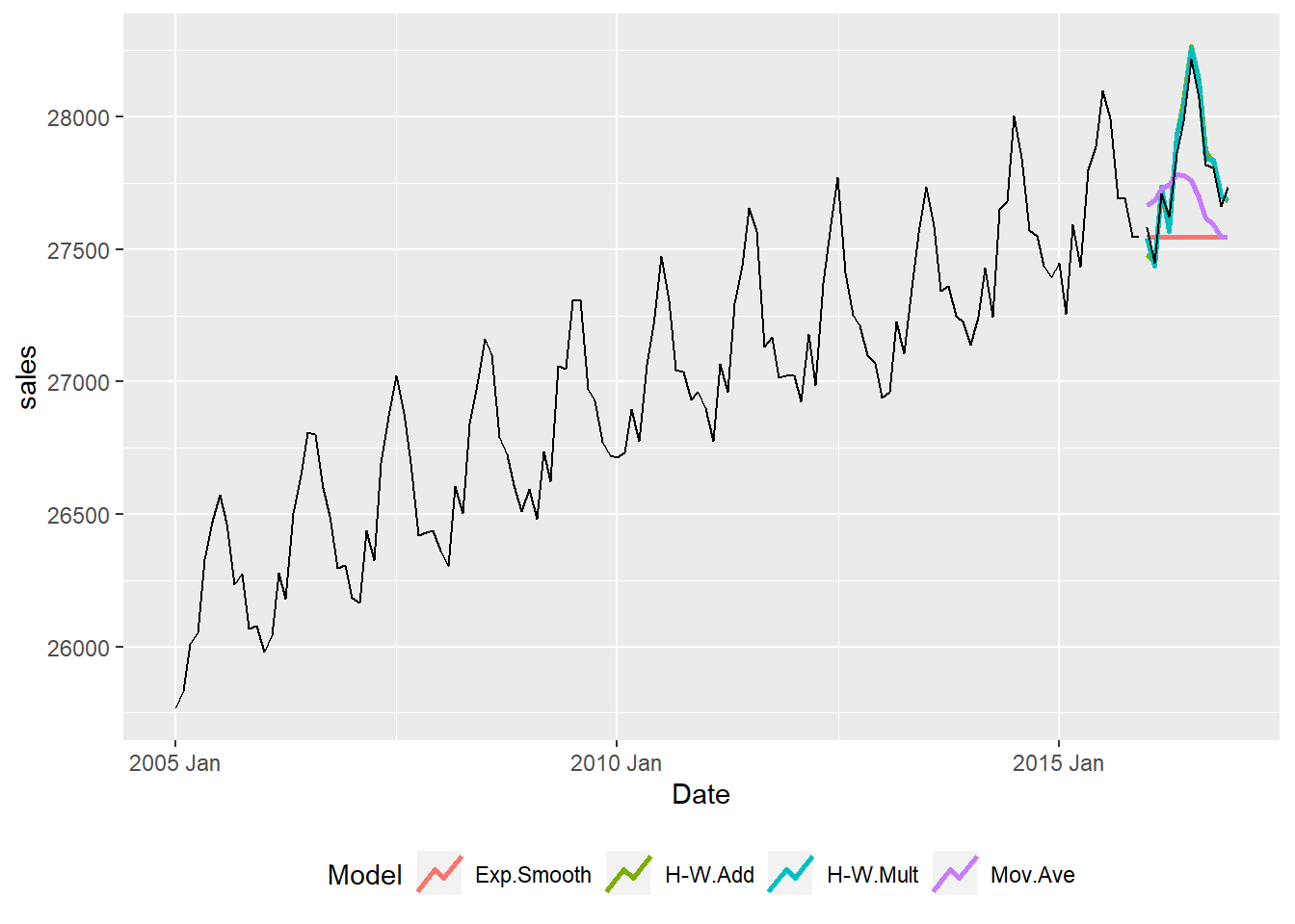
tsplot(msales,  # Dataframe
       "t",     # Date variable
       "sales", # Measure variable
       "ym",    # Date type
       12)      # Holdout periods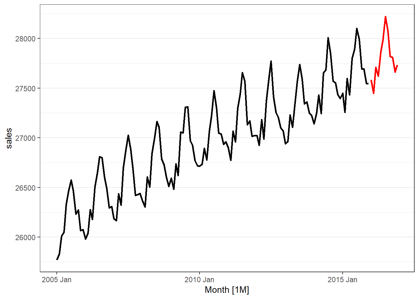

tsplot(qsales, "t", "sales", "yq", 8)

11.3 naivefc User Defined Function

• Usage: naivefc(data, tvar="", obs="", datetype=c("ym", "yq", "yw"), h= )
  • data is the name of the dataframe with the time variable and measure variable
  • tvar is the variable that identifies the time period (in quotes)
  • obs is the variable that identifies the measure (in quotes)
  • datetype can be one of three options:
    • "ym" if the time period is year-month
    • "yq" if the time period is year-quarter
    • "yw" if the time period is year-week
  • h is an integer indicating the number of holdout/forecast periods
• NOTE 1: The results of this function should be saved to an object. When doing so, the following objects are returned:
  • $plot contains the naive methods plot
  • $acc contains the accuracy measures
  • $fcresplot contains a plot of the holdout period residuals
  • $fcresid is a dataframe of the holdout period residuals (seldom used separately)
• Note 2: The model names are:
  • Naive for the naive model
  • Naive.Drift for the naive model with drift
  • Seas.Naive for the seasonal naive model
  • Seas.Naive.Drift for the seasonal naive model with drift

naive <- naivefc(msales, "t", "sales", "ym", 12)
naive$plot

naive$acc

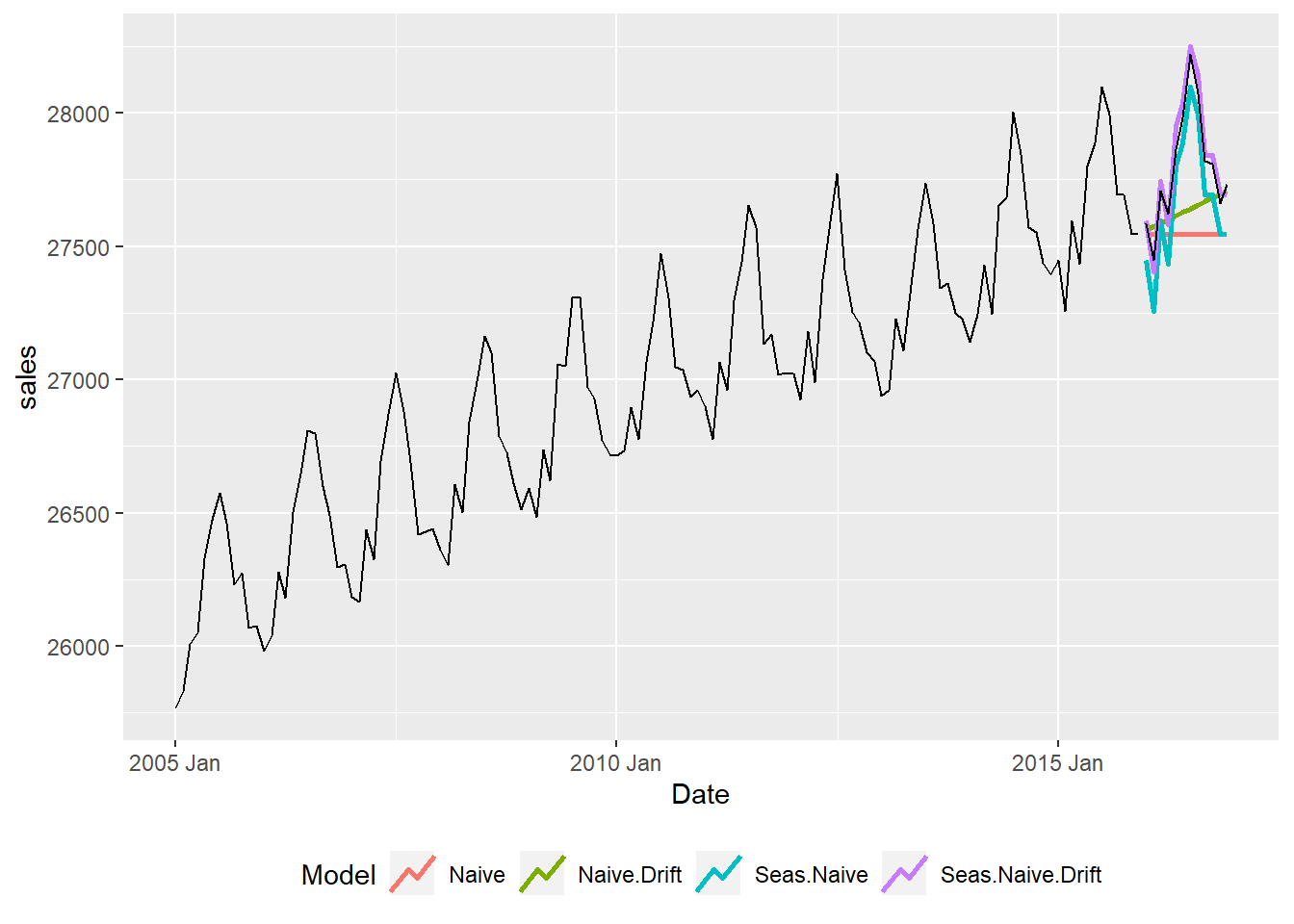
             Model    RMSE     MAE  MAPE
1            Naive 323.496 263.917 0.945
2      Naive.Drift 253.103 185.868 0.665
3       Seas.Naive 133.710 127.417 0.459
4 Seas.Naive.Drift  45.769  41.417 0.149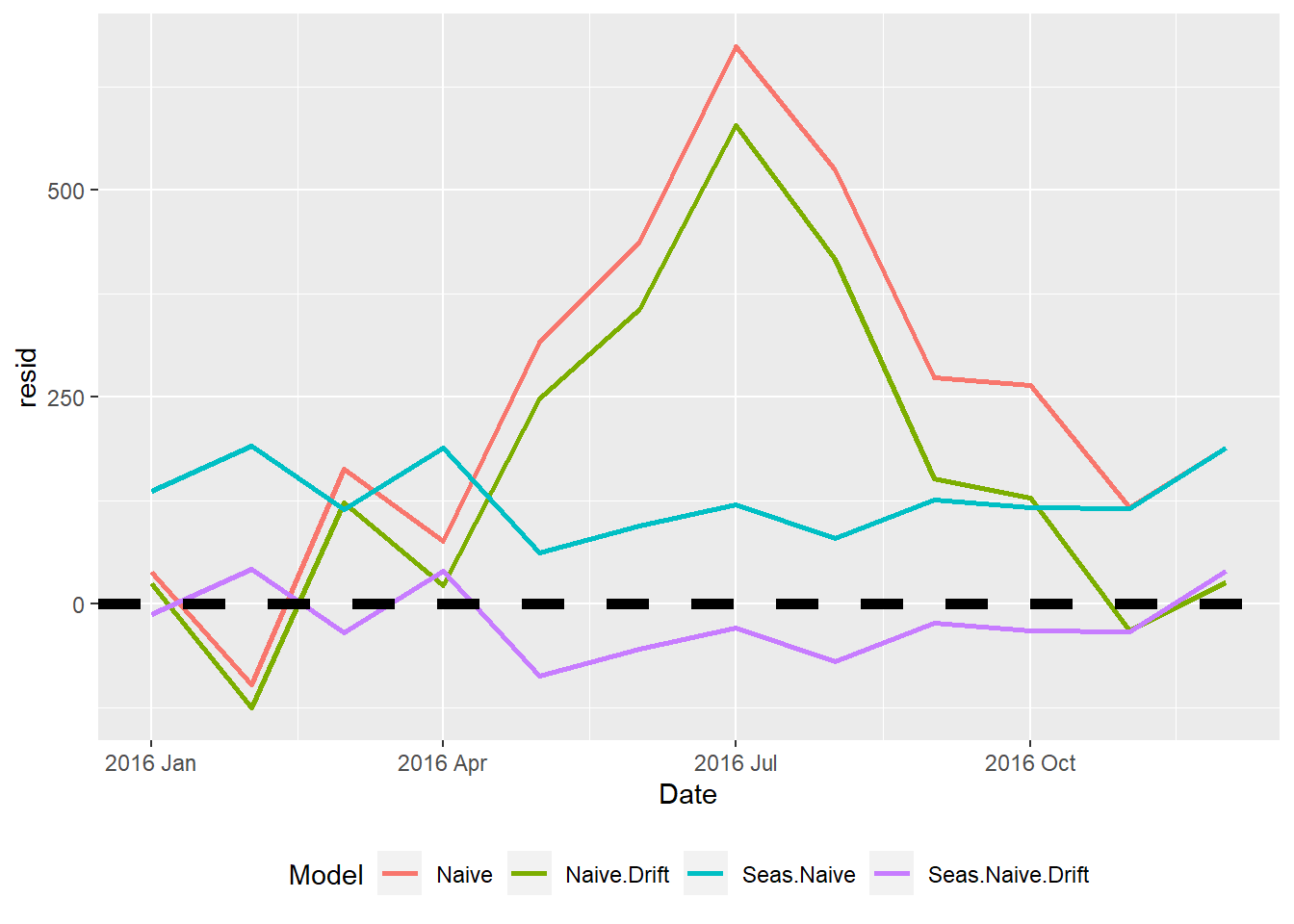

naive$fcresplot

11.4 smoothfc User Defined Function

• Usage: smoothfc(data, tvar="", obs="", datetype=c("ym", "yq", "yw"), h= )
  • data is the name of the dataframe with the time variable and measure variable
  • tvar is the variable that identifies the time period (in quotes)
  • obs is the variable that identifies the measure (in quotes)
  • datetype can be one of three options:
    • "ym" if the time period is year-month
    • "yq" if the time period is year-quarter
    • "yw" if the time period is year-week
  • h is an integer indicating the number of holdout/forecast periods
• NOTE 1: The results of this function should be saved to an object. When doing so, the following objects are returned:
  • $plot contains the smoothing methods plot
  • $acc contains the accuracy measures
  • $fcresplot contains a plot of the holdout period residuals
  • $fcresid is a dataframe of the holdout period residuals (seldom used separately)
• Note 2: The model names are:
  • Mov.Ave for the moving average model
  • Exp.Smooth for the exponential smoothing model
  • H-W.Add for the Holt-Winters Additive model
  • H-W.Mult for Hold-Winters Multiplicative model

smooth <- smoothfc(msales, "t", "sales", "ym", 12)
smooth$plot

smooth$acc

       Model    RMSE     MAE  MAPE
1 Exp.Smooth 323.495 263.915 0.945
2    H-W.Add  54.469  46.754 0.168
3   H-W.Mult  43.857  40.626 0.146
4    Mov.Ave 225.685 191.245 0.686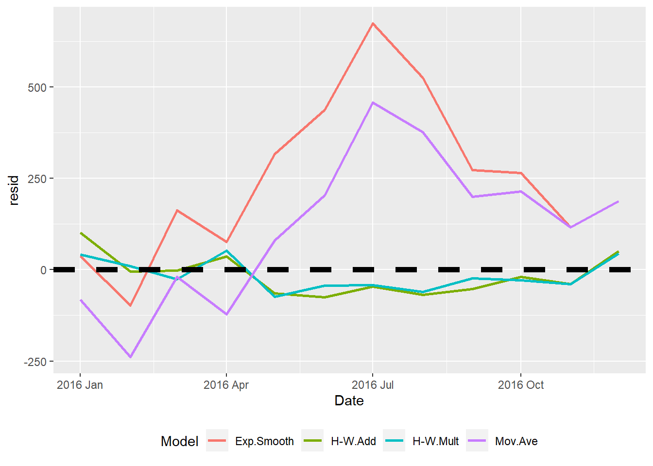

smooth$fcresplot

11.5 linregfc User Defined Function

• Usage: linregfc(data, tvar="", obs="", datetype=c("ym", "yq", "yw"), h= )
  • data is the name of the dataframe with the time variable and measure variable
  • tvar is the variable that identifies the time period (in quotes)
  • obs is the variable that identifies the measure (in quotes)
  • datetype can be one of three options:
    • "ym" if the time period is year-month
    • "yq" if the time period is year-quarter
    • "yw" if the time period is year-week
  • h is an integer indicating the number of holdout/forecast periods
• NOTE 1: The results of this function should be saved to an object. When doing so, the following objects are returned:
  • $plot contains the regression methods plot
  • $acc contains the accuracy measures
  • $fcresplot contains a plot of the holdout period residuals
  • $fcresid is a dataframe of the holdout period residuals (seldom used separately)
• Note 2: The model names are:
  • Lin.Reg.Trend for the linear regression with trend model
  • Line.Reg.Seas.Trend for linear regression with trend and seasonality model

linreg <- linregfc(msales, "t", "sales", "ym", 12)
linreg$plot

linreg$acc

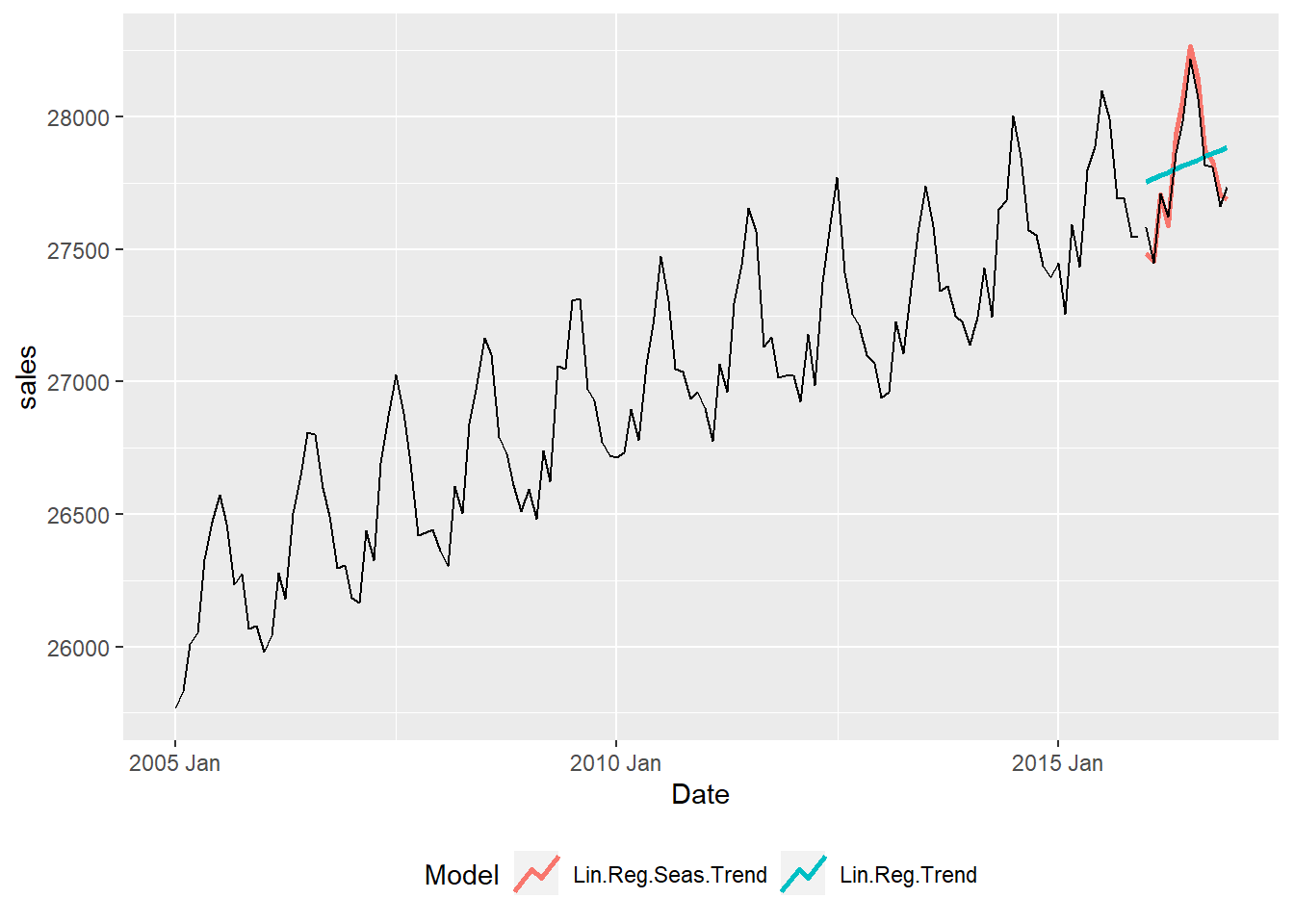
               Model    RMSE     MAE  MAPE
1 Lin.Reg.Seas.Trend  55.212  47.898 0.172
2      Lin.Reg.Trend 199.198 168.985 0.607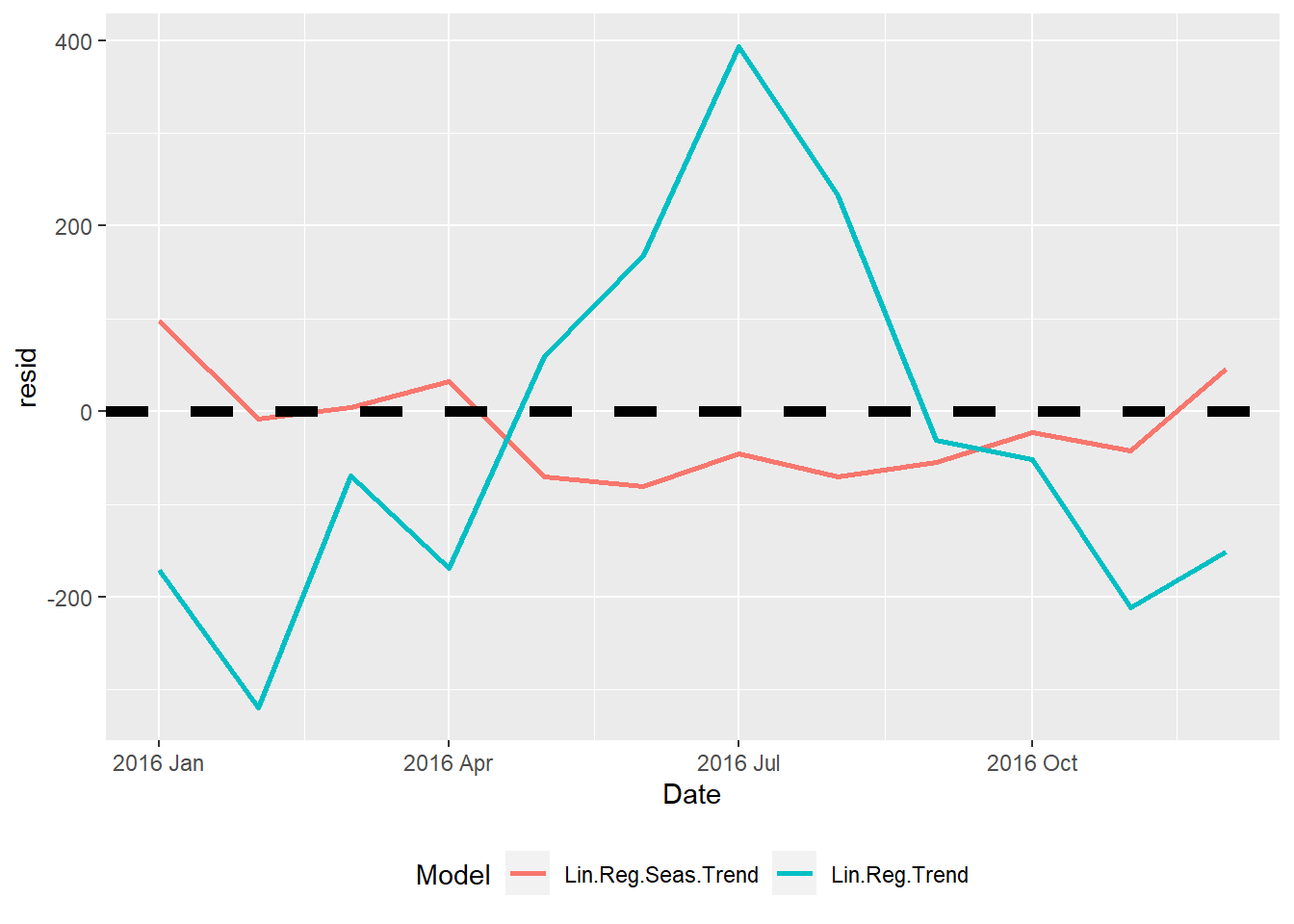

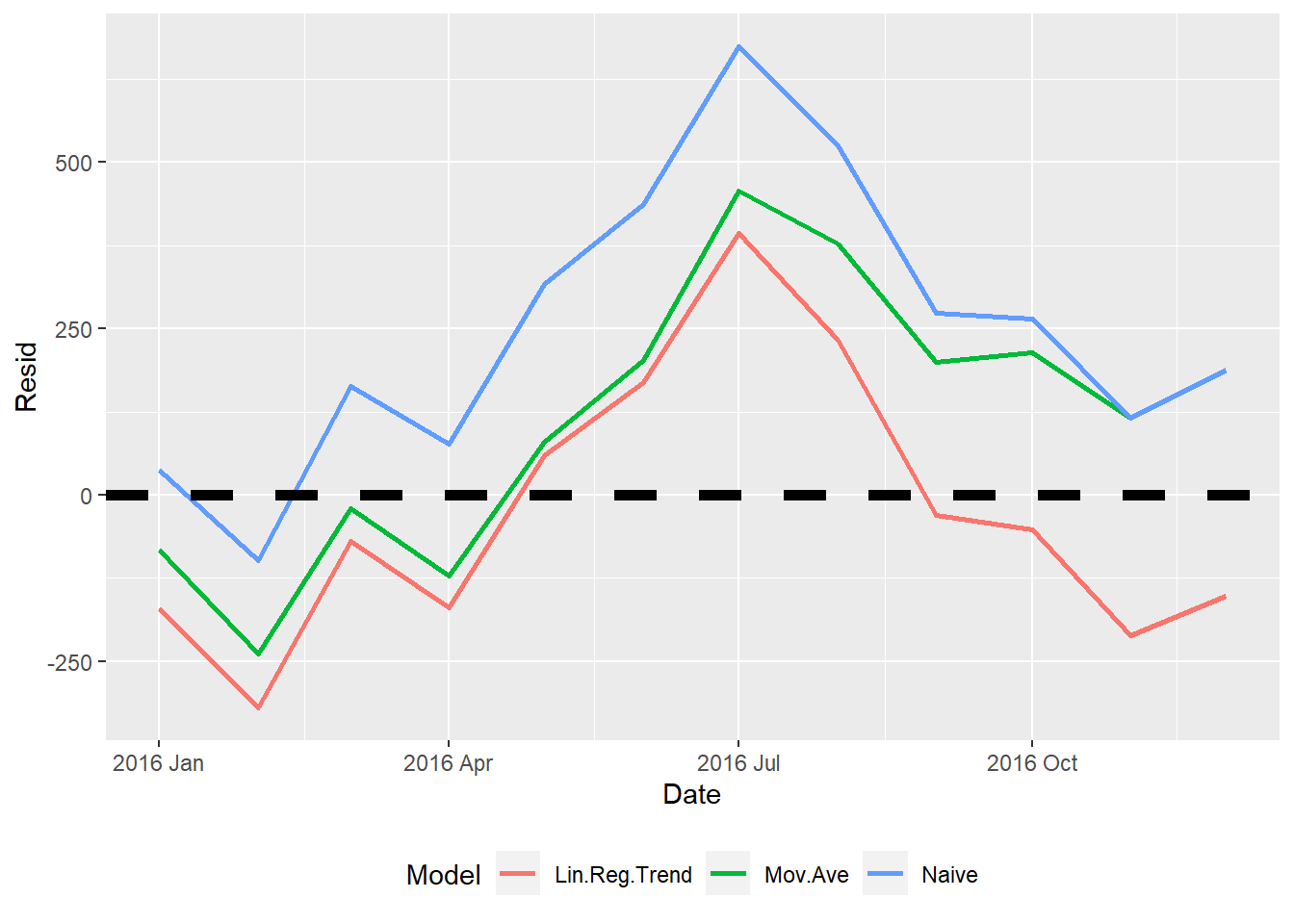
linreg$fcresplot

11.6 fccompare User Defined Function

• Usage: fccompare(results, models)
  • results is a list of the stored methods results; create the list with the list function, such as:
    results <- list(naive, smooth, linreg)
  • models is a vector of the models you want to compare; create the vector with the c() function, such as:
    models <- c("Naive", "Mov.Ave", "Lin.Reg.Trend")
• NOTE 1: The function returns two items that will be directly displayed or can be saved to an object:
  • $acc contains the accuracy measures
  • $fcresplot contains a plot of the holdout period residuals

results <- list(naive, smooth, linreg)
models <- c("Naive", "Mov.Ave", "Lin.Reg.Trend")
fccompare(results, models)

$acc
           Model    RMSE     MAE  MAPE
1          Naive 323.496 263.917 0.945
8        Mov.Ave 225.685 191.245 0.686
10 Lin.Reg.Trend 199.198 168.985 0.607

$fcresplot