Chapter 6 Principal Components Analysis

Sources for this chapter:

R for Marketing Research and Analytics, Second Edition (2019). Chris Chapman and Elea McDonnell Feit
- http://r-marketing.r-forge.r-project.org/index.html

Data for this chapter:

The greekbrands data is used from the MKT4320BGSU course package. Load the package and use the data() function to load the data.
```
# Load the course package
library(MKT4320BGSU)
# Load the data
data(greekbrands)
```

6.1 Introduction

Base R is typically sufficient for performing the basics of principal components analysis, but to get some of the outputs required more easily and more efficiently, I have created a user defined function, which is part of the MKT4320BGSU package.

pcaex provides an eigenvalue table, scree plot, unrotated and rotated factor loading tables, and the principal components R object

6.2 Base R

6.2.1 `prcomp()` function

The prcomp() function performs PCA

Usage: prcomp(formula, data=, scale=TRUE, rank=) where:
- formula is a formula with no response variables, but rather only the numeric variables to be included if not all variables in data are to be included
  - No response variable means the formula is written as:
    ~var1 + var2 + var3 + ... + var4
- data= is the name of the dataframe
- scale=TRUE standardizes the variables before running the PCA
- rank= is the number of components to retain; default is all
When saved to an object, the following components are saved:
- $sdev is the standard deviations of the principal components (i.e., the square roots of the eigenvalues)
- $rotation is the unroated factor loadings
- $x is the factor scores

Example: perform PCA on $serious$, $fun$, $bargain$, $trendy$, and $value$ with only two components retained

pcaout <- prcomp(~serious+fun+bargain+trendy+value, # Variables to include
                 data=greekbrands,  # Data frame to use
                 scale=TRUE,   # Standardize the variables
                 rank=2)   # Retain only first two components

6.2.2 Eigenvalue table

To get the eigenvalue table, we must square the $sdev component of the PCA object

eigtable <- data.frame(components=seq(1:5), # column with component #'s
                       pcaout$sdev^2)  # Eigenvalues
eigtable

  components pcaout.sdev.2
1          1     2.0722697
2          2     1.2747721
3          3     0.8111322
4          4     0.5913799
5          5     0.2504461

6.2.3 Unrotated loadings

Unrotated factor loadings are in the $rotation component of the PCA object

pcaout$rotation

                 PC1         PC2
serious  0.006484917 -0.73514845
fun     -0.179503188  0.65827780
bargain  0.596338877  0.07600771
trendy  -0.469318304 -0.14191980
value    0.625984684  0.01756980

Rotated loadings

Rotated loadings are not automatically created. Instead, we must use the varimax(pcaobject$rotation)$loadings command to obtain them. By default, only rotated loadings greater than 0.4 are shown.

varimax(pcaout$rotation)$loadings


Loadings:
        PC1    PC2   
serious -0.101 -0.728
fun             0.677
bargain  0.601       
trendy  -0.485       
value    0.622       

               PC1 PC2
SS loadings    1.0 1.0
Proportion Var 0.2 0.2
Cumulative Var 0.2 0.4

6.3 User Defined Function

The pcaex user defined function can produce the results with one or two passes of the function
- Requires the following packages:
  - ggplot2
  - dplyr
The results should be saved to an object
Usage: pcaex(data, group="", pref="", comp=) where:
- data is the PCA variable data
- group="" is the name of the grouping variable
  - Can be excluded if no grouping variable
- pref="" is the name of the preference variable
  - Can be excluded if no preference variable
- comp= is the number of components to retain
  - Default is NULL if all components are wanted
Objects returned:
- If comp is NOT provided:
  - Scree plot ($plot)
  - Table of eigenvalues ($table)
- If comp is provided:
  - Table of eigenvalues ($table)
  - Unrotated factor loading table ($unrotated)
  - Rotated factor loading table ($rotated)
  - PCA object ($pcaobj)
When a group= variable is provided, the PCA will be performed on an aggregated data frame (i.e., mean values by group)

6.3.1 Preparation

We need to pass a data frame to the user defined function containing the variables to be used (and maybe a preference and group/brand variable, see below)
- In our class, the data set will often be used for creating a perceptual map, so we may also have a grouping variable (e.g., brand or product name) and a preference variable
- Package dplyr is usually the best tool for this
For this tutorial, we will perform a PCA using the greekbrands dataframe
- We will use only the following attributes:
  - $perform$, $leader$, $fun$, $serious$, $bargain$, $value$
  - The data also has a preference variable, $pref$ and a group variable, $brand$, but we do not always want to use them.

library(dplyr)
# Store variables selected to 'pcadata1' (WITHOUT group and pref variables)
pcadata1 <- greekbrands %>%   
    select(perform, leader, fun, serious, bargain, value)

# Store variables selected to 'pcadata2' (INCLUDES group and pref variables)
pcadata2 <- greekbrands %>%   
    select(perform, leader, fun, serious, bargain, value,
           pref, brand)

6.3.2 Examples

6.3.2.1 WITHOUT `group=` or `pref=` options

All components

    gb1.all <- pcaex(pcadata1)    # PCA data created earlier
    # Do not include 'comp' to get all components
    
    # Call gb1.all$table to get eigenvalue table
    gb1.all$table

  Component Eigenvalue Difference Proporation Cumulative
1         1     2.2293     0.5454      0.3716     0.3716
2         2     1.6839     0.8876      0.2806     0.6522
3         3     0.7963     0.1545      0.1327     0.7849
4         4     0.6418     0.2433      0.1070     0.8919
5         5     0.3985     0.1484      0.0664     0.9583
6         6     0.2501         NA      0.0417     1.0000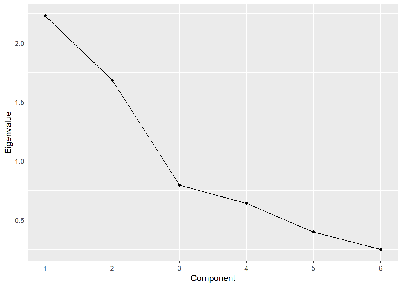

    # Call gb1.all$plot to get scree plot
    gb1.all$plot

Two components

    gb1.2comp <- pcaex(pcadata1,    # PCA data created earlier
                       comp=2)   # Request 2 components
    
    # Call gb1.2comp$unrotated to get unrotated factor loadings
    gb1.2comp$unrotated

            PC1     PC2 Unexplained
perform  0.4683  0.1568      0.4697
leader   0.5336  0.2093      0.2914
fun     -0.3774 -0.0522      0.6778
serious  0.4760  0.2589      0.3821
bargain  0.2228 -0.6689      0.1359
value    0.2780 -0.6438      0.1298

    # Call gb1.2comp$rotated to get rotated factor loadings
    gb1.2comp$rotated

            PC1     PC2 Unexplained
perform  0.4933 -0.0233      0.4697
leader   0.5732  0.0021      0.2914
fun     -0.3708  0.0879      0.6778
serious  0.5374  0.0691      0.3821
bargain -0.0343 -0.7042      0.1359
value    0.0263 -0.7007      0.1298

6.3.2.2 WITH `group=` or `pref=` options

All components

    gb2.all <- pcaex(pcadata2,    # PCA data created earlier
                     group="brand",   # Grouping variable
                     pref="pref")    # Preference variable
    # Do not include 'comp' to get all components
    # Call gb2.all$table to get eigenvalue table
    gb2.all$table

  Component Eigenvalue Difference Proporation Cumulative
1         1     3.4180     1.5468      0.5697     0.5697
2         2     1.8712     1.4213      0.3119     0.8815
3         3     0.4500     0.2527      0.0750     0.9565
4         4     0.1973     0.1567      0.0329     0.9894
5         5     0.0405     0.0175      0.0068     0.9962
6         6     0.0231         NA      0.0038     1.0000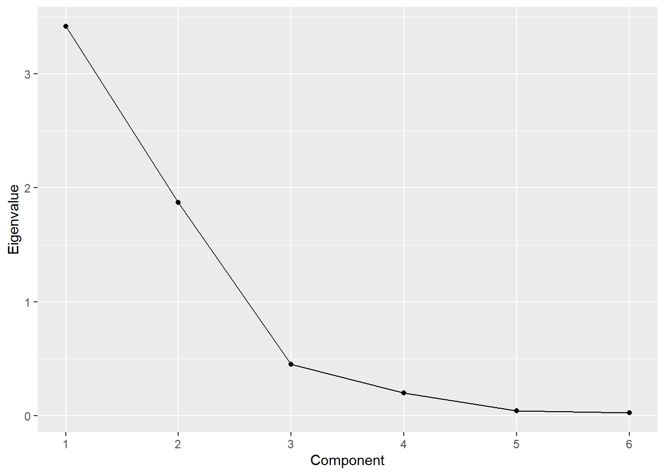

    # Call gb2.all$plot to get scree plot
    gb2.all$plot

Two components

    gb2.2comp <- pcaex(pcadata2,    # PCA data created earlier
                       group="brand",   # Grouping variable
                       pref="pref",    # Preference variable
                       comp=2)   # Request 2 components

    # Call gb2.2comp$unrotated to get unrotated factor loadings
    gb2.2comp$unrotated

            PC1     PC2 Unexplained
perform  0.4455  0.0934      0.3054
leader   0.4970  0.1817      0.0941
fun     -0.5005 -0.0351      0.1416
serious  0.4712  0.2503      0.1239
bargain  0.1718 -0.6815      0.0299
value    0.2293 -0.6557      0.0159

    # Call gb2.2comp$rotated to get rotated factor loadings
    gb2.2comp$rotated

            PC1     PC2 Unexplained
perform  0.4533 -0.0409      0.3054
leader   0.5284  0.0284      0.0941
fun     -0.4889  0.1127      0.1416
serious  0.5238  0.1016      0.1239
bargain -0.0350 -0.7020      0.0299
value    0.0275 -0.6941      0.0159