Chapter 3 Linear Regression
Sources for this chapter:
- R for Marketing Research ad Analytics, Second Edition (2019). Chris Chapman and Elea McDonnell Feit
- ggplot2: https://ggplot2.tidyverse.org/
Data for this chapter:
Once again, the
airlinesatdata is used from theMKT4320BGSUcourse package. Load the package and use thedata()function to load the data.
3.1 Introduction
Base R is typically sufficient for performing most regression tasks. Some additional packages may be used for “prettier” tables or extracting results to make useful plots.
3.2 The lm() Function
- Basic linear regression is performed using the
lm()function. - Usage:
lm(formula, data) - In R, a formula is represented by dependent variables on the left side separated from the independent variables on the right side by a tilde(
~), such as:dv ~ iv1 + iv2- For interactions between independent variables, use either
*or:*will include the interaction term AND each main effect:will include ONLY the iteraction term- Examples:
y ~ x1 + x2*x3is the same as:
\(y=x_1+x_2+x_3+(x_2\times x_3)\)y ~ x1 + x2:x3is the same as:
\(y=x_1+(x_2\times x_3)\)y ~ x1 + x2 + x2:x3is the same as:
\(y=x_1+x_2+(x_2\times x_3)\)
- For interactions between independent variables, use either
Video Tutorial: lm() - Basic Usage
If
lm()is run by itself, R only outputs the coefficientsCall: lm(formula = nps ~ age + nflights, data = airlinesat) Coefficients: (Intercept) age nflights 6.786100 0.016985 -0.009112Table 3.1: Coefficients from
lm()callHowever, if the results of the
lm()call are assigned to an object, thesummary()function can be used to get much more detailed outputCall: lm(formula = nps ~ age + nflights, data = airlinesat) Residuals: Min 1Q Median 3Q Max -6.988 -1.316 0.440 1.725 7.682 Coefficients: Estimate Std. Error t value Pr(>|t|) (Intercept) 6.786100 0.310554 21.852 < 2e-16 *** age 0.016985 0.005815 2.921 0.00357 ** nflights -0.009112 0.003529 -2.582 0.00995 ** --- Signif. codes: 0 '***' 0.001 '**' 0.01 '*' 0.05 '.' 0.1 ' ' 1 Residual standard error: 2.313 on 1062 degrees of freedom Multiple R-squared: 0.01591, Adjusted R-squared: 0.01406 F-statistic: 8.587 on 2 and 1062 DF, p-value: 0.0001997Table 3.2: Summary results from
lm()call
To get standardized beta coefficients, use the
lm_beta()function from theMKT4320BGSUcourse package.Std.Beta (Intercept) 0.0000 age 0.0895 nflights -0.0791Table 3.3: Standardized Beta Coefficients
Video Tutorial: lm() - Standardized Beta Coefficients
For “nicer” looking results, the
tab_modelfunction from thesjPlotpackage can be usednps
Predictors
Estimates
CI
Statistic
p
(Intercept)
6.79
6.18 – 7.40
21.85
<0.001
age
0.02
0.01 – 0.03
2.92
0.004
nflights
-0.01
-0.02 – -0.00
-2.58
0.010
Observations
1065
R2 / R2 adjusted
0.016 / 0.014
Table 3.4: Summary results from
lm()usingsjPlotpackage- Standardized beta coefficients can also be obtained
library(sjPlot)
tab_model(model1,   # Saved object from before
     show.stat=TRUE, # Display t-statistic
     show.std=TRUE, # Display standardized beta coefficients
     show.ci=FALSE) # Remove confidence intervals for cleaner table
nps
Predictors
Estimates
std. Beta
Statistic
p
(Intercept)
6.79
0.00
21.85
<0.001
age
0.02
0.09
2.92
0.004
nflights
-0.01
-0.08
-2.58
0.010
Observations
1065
R2 / R2 adjusted
0.016 / 0.014
Table 3.5: Summary results from
lm()usingsjPlotpackage
Video Tutorial: lm() - Results using the sjPlot Package
- For “nicer” looking results, the
summfunction from thejtoolspackage can be used- NOTE:
jtoolsis not available in BGSU’s Virtual Computing Lab
library(jtools)
summ(model1,   # Saved object from before
     digits=4) # How many digits to display in each column
Observations 1065 Dependent variable nps Type OLS linear regression F(2,1062) 8.5875 R² 0.0159 Adj. R² 0.0141 Est. S.E. t val. p (Intercept) 6.7861 0.3106 21.8516 0.0000 age 0.0170 0.0058 2.9208 0.0036 nflights -0.0091 0.0035 -2.5822 0.0100 Standard errors: OLS Table 3.6: Summary results from lm()usingjtoolspackage- Standardized beta coefficients can also be obtained
library(jtools)
summ(model1,   # Saved object from before
     digits=4, # How many digits to display in each column
     scale=TRUE,  # Standardize the IVs
     transform.response=TRUE)  # Standarize the DV
Observations 1065 Dependent variable nps Type OLS linear regression F(2,1062) 8.5875 R² 0.0159 Adj. R² 0.0141 Est. S.E. t val. p (Intercept) 0.0000 0.0304 0.0000 1.0000 age 0.0895 0.0306 2.9208 0.0036 nflights -0.0791 0.0306 -2.5822 0.0100 Standard errors: OLS; Continuous variables are mean-centered and scaled by 1 s.d. Table 3.7: Standardized Beta Coefficients from lm()usingjtoolspackage - NOTE:
3.3 Prediction
The function predict.lm() can be used to predict the DV based on values of the IVs. This function is used in the margin plots covered in the next two sections. To use this function, we must pass a data frame of values to the function, where the data frame contains ALL of the IVs and the value for each IV that we want.
Suppose we wanted to predict, with a confidence interval, the nps of someone that is 45 years old and had 25 flights on the airline, and also someone that is 25 years old and had 45 flights on the airline. First, we create the data frame of values (see 1.6.2.1):
  age nflights
1  45       25
2  25       45
Second, the data frame is passed to the predict.lm() function with confidence intervals requested:
predict.lm(model1,   # The model we are using to predict
           values,   # The data frame of values to predict with
           interval="confidence")   # Request confidence interval
fit lwr upr
1 7.322601 7.153951 7.491252
2 6.800657 6.431058 7.1702553.4 Margin Plots (Manual Process)
In R, margin plots are a multistep process:
- Use the
predictorEffectfunction from theeffectspackage to create a data frame of predicted values for different values of the focal variable.- For continuous focal variables, predictions will be made for 50 evenly-spaced values of the focal variable at mean values of the other variables.
- If the model has an interaction between a continuous focal variable and a factor variable, predictions will be made for each level of the factor variable.
- If the model has an interaction between a continuous focal variable and another continuous variable, predictions will be made for 5 evenly-spaced values of the other continuous variable.
- For factor focal variables, predictions will be made for each level of the factor variable at mean values of the other variables.
- If the model has an interaction between a factor focal variable and a continuous variable, predictions will be made for 5 evenly-spaced values of the the continuous variable.
- If the model has an interaction between a factor focal variable and another factor variable, predictions will be made for every combination of the two factor variables.
- By default, the dataframe will contain the predicted value (
fit) and values for a \(95\%\) confidence interval (lowerandupper)
- For continuous focal variables, predictions will be made for 50 evenly-spaced values of the focal variable at mean values of the other variables.
- Use
ggplotto create the margin plot
Video Tutorial: lm() - Introduction to Margin Plots
3.4.1 Continuous IV (No Interaction)
library(effects)  # Load package 'effects'

# Want to predict 'nps' for different levels of 'age'
age.pred <- data.frame(predictorEffect("age",  # Focal variable
                                       model1))

# Use 'age.pred' for margin plot
age.pred %>%
   ggplot(aes(x=age,   # Age on x-axis
              y=fit)) +   # 'nps' prediction on y-axis
   geom_line(size=1) +   # Draw predicted line
   geom_ribbon(aes(ymin=lower,  # Draws the confidence interval bands
                   ymax=upper),
               alpha=0.2) + # Sets transparency level
   labs(x="Age", y="Linear Prediciton")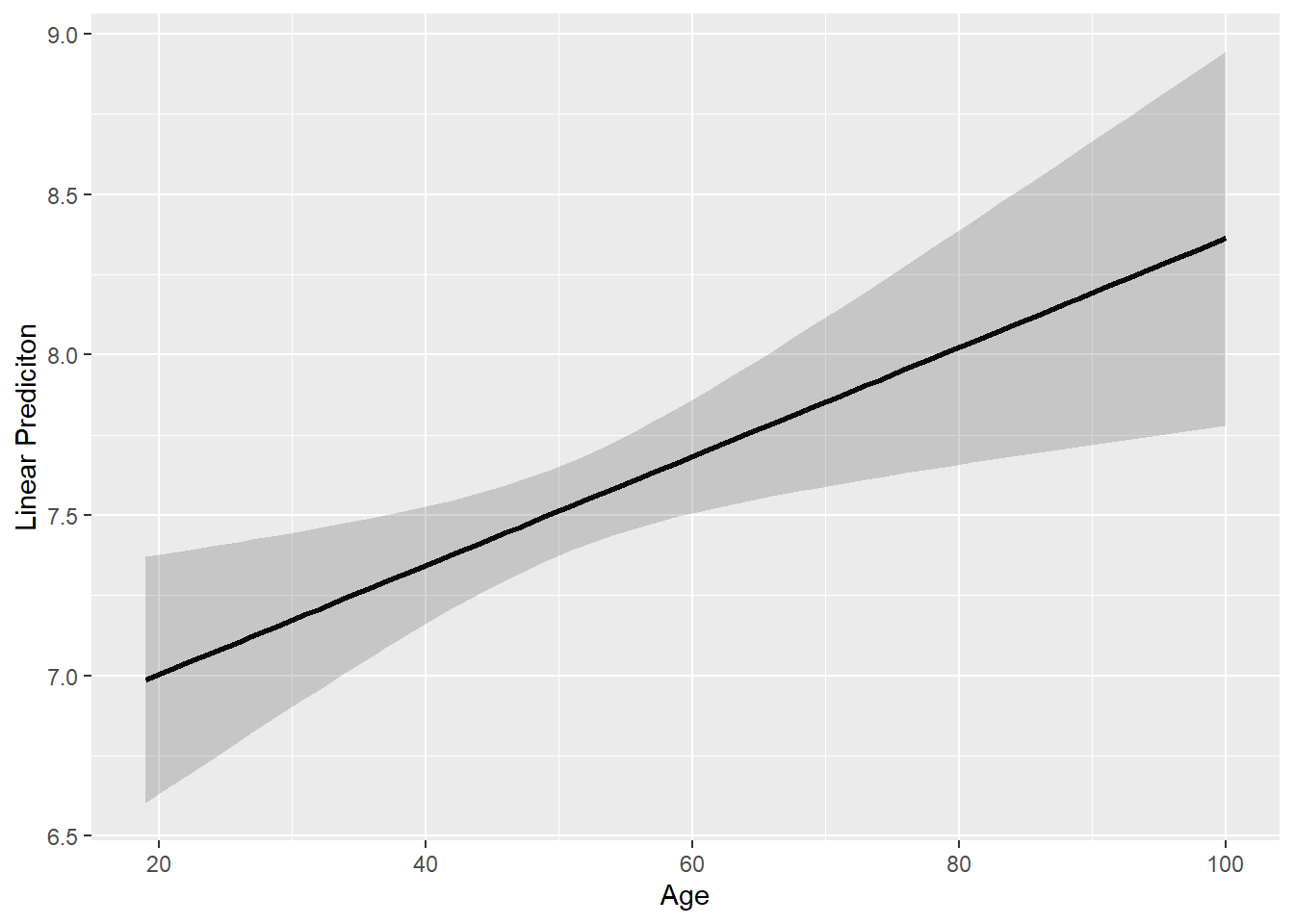
Figure 3.1: Margin plot (continuous IV)
Video Tutorial: lm() - Margin Plots for Continuous IV with no Interaction
3.4.2 Separate Margin Plots (No Interaction)
- If creating separate plots for each continuous IV, it is best to have the prediction (y) variable have the same scale
- Doing so might take some trial and error after looking at graphs once
- Use the function
plot_grid()from thecowplotpackage to make the plots appear in the same figure- Save each plot as an object, then pass the objects to
plot_grid()
- Save each plot as an object, then pass the objects to
library(cowplot)
# Using dataframe from previous chunk, ask for min/max of the 95% CI adjust axis
min(age.pred$lower)
[1] 6.601996[1] 8.944869# Save previous plot (for 'age') as plot 1
plot1 <- age.pred %>%
ggplot(aes(x=age,y=fit)) +
geom_line(size=1) +
geom_ribbon(aes(ymin=lower, ymax=upper), alpha=0.2) +
labs(x="Age", y="Linear Prediciton") +
scale_y_continuous(limits=c(5.25,9.25)) # Set scale limits for y-axis
# Create second plot for 'nflights' using procedure above
# Because of outliers in 'nflights', use the 'focal.levels=' option for more
# realistic predictions
nflights.pred <- data.frame(predictorEffect("nflights", # Focal variable
model1,
focal.levels=seq(0,150,3)))
min(nflights.pred$lower)[1] 5.319659[1] 7.809707plot2 <- nflights.pred %>%
ggplot(aes(x=nflights, y=fit)) +
geom_line(size=1) +
geom_ribbon(aes(ymin=lower,ymax=upper),alpha=0.2) +
labs(x="Number of Flights", y="Linear Prediciton") +
scale_y_continuous(limits=c(5.25,9.25)) # Set scale limits for y-axis
# Use 'cowplot' function 'plot_grid' to combine plots
cowplot::plot_grid(plot1,plot2)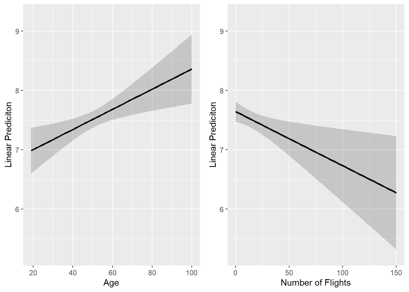
Figure 3.2: Separate margin plots (continuous factor IVs)
Video Tutorial: lm() - Side-by-Side Margin Plots using cowplot Package
3.4.3 Factor IV (No Interaction)
- Margin plots for a factor IV without an interaction consist of a point and \(95\%\) confidence interval error bars
# Run new model with flight_purpose included
model2 <- lm(nps ~ age + nflights + flight_purpose, airlinesat)
summary(model2)
Call:
lm(formula = nps ~ age + nflights + flight_purpose, data = airlinesat)

Residuals:
   Min     1Q Median     3Q    Max
-7.130 -1.160  0.521  1.808  6.306

Coefficients:
                       Estimate Std. Error t value Pr(>|t|)
(Intercept)            6.644742   0.313158  21.218  < 2e-16 ***
age                    0.014749   0.005844   2.524  0.01175 *
nflights              -0.006540   0.003624  -1.805  0.07140 .
flight_purposeLeisure  0.433007   0.147317   2.939  0.00336 **
---
Signif. codes:  0 '***' 0.001 '**' 0.01 '*' 0.05 '.' 0.1 ' ' 1

Residual standard error: 2.304 on 1061 degrees of freedom
Multiple R-squared:  0.02386,   Adjusted R-squared:  0.0211
F-statistic: 8.646 on 3 and 1061 DF, p-value: 1.136e-05# Create data frame with values to be plotted
fp.pred <- data.frame(predictorEffect("flight_purpose", model2))
# Create plot
fp.pred %>%
ggplot(aes(x=flight_purpose, y=fit,
group=1)) + # Need to draw line between points
geom_point(size=4) +
geom_line(color="orange") +
geom_errorbar(aes(ymin=lower, ymax=upper), width=.5) +
labs(x="Flight Purpose", y="Linear Prediction")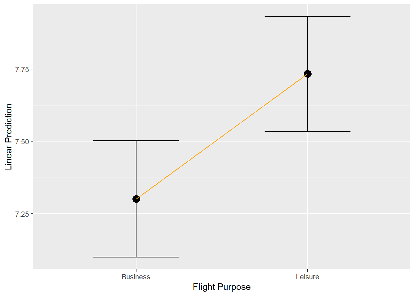
Figure 3.3: Margin plot (factor IV)
Video Tutorial: lm() - Margin Plots for Factor IV with No Interaction
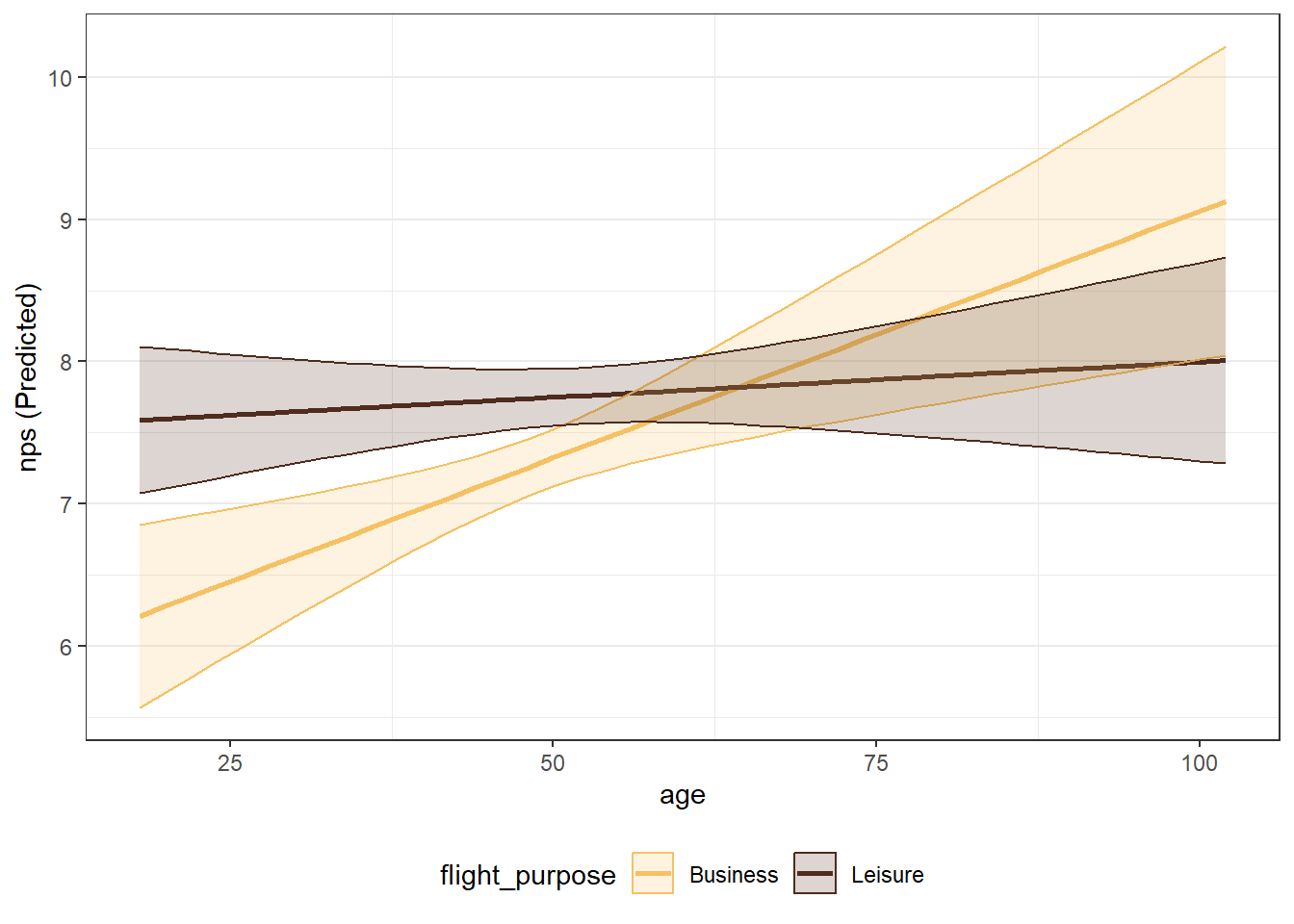
3.4.4 Continuous IV (Interaction with Factor IV)
- Margin plots when for a continuous IV interaction with a factor IV are done in much the same way, but require an
aes(color=factor, fill=factor)to produce different colored lines for each level of the factor
# Run new model with 'age' and 'flight_purpose' interaction
model3 <- lm(nps ~ age*flight_purpose + nflights, airlinesat)
summary(model3)
Call:
lm(formula = nps ~ age * flight_purpose + nflights, data = airlinesat)

Residuals:
    Min      1Q  Median      3Q     Max
-6.9177 -1.0298  0.3193  1.8402  6.1721

Coefficients:
                           Estimate Std. Error t value Pr(>|t|)
(Intercept)                5.675998   0.510101  11.127  < 2e-16 ***
age                        0.034704   0.010148   3.420 0.000651 ***
flight_purposeLeisure      1.912145   0.632942   3.021 0.002579 **
nflights                  -0.006487   0.003616  -1.794 0.073088 .
age:flight_purposeLeisure -0.029724   0.012372  -2.403 0.016450 *
---
Signif. codes:  0 '***' 0.001 '**' 0.01 '*' 0.05 '.' 0.1 ' ' 1

Residual standard error: 2.299 on 1060 degrees of freedom
Multiple R-squared:  0.02915,   Adjusted R-squared:  0.02549
F-statistic: 7.957 on 4 and 1060 DF, p-value: 2.551e-06# Create data frame with values to be plotted
age.pred <- data.frame(predictorEffect("age", model3))
# Create plot
age.pred %>%
ggplot(aes(x=age, y=fit,
color=flight_purpose, fill=flight_purpose)) + # color based on factor
geom_line(size=1) + # Draw predicted line
geom_ribbon(aes(ymin=lower, # Draws the confidence interval bands
ymax=upper),
alpha=0.2) + # Sets transparency level
labs(x="Age", y="Linear Prediciton", color="Flight Purpose", fill="Flight Purpose") +
theme(legend.position="bottom")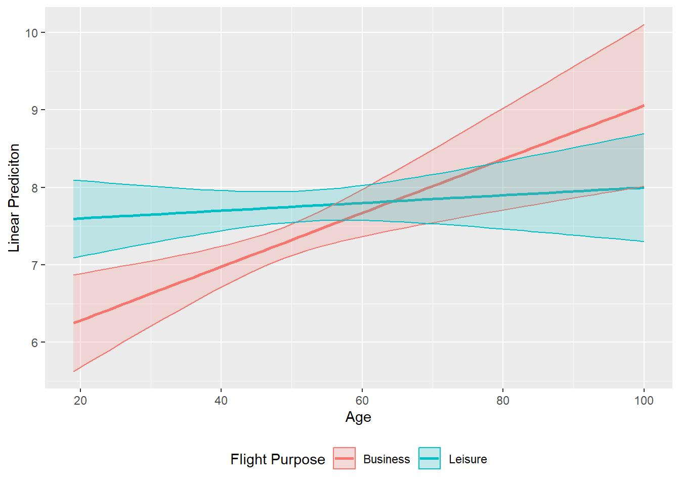
Figure 3.4: Margin plot (continuous IV with factor IV interaction)
Video Tutorial: lm() - Margin Plots for Continuous IV with Factor IV Interaction
3.4.5 Factor IV (Interaction with Continuous IV)
- Margin plots for a factor IV interaction with a continuous IV are done in much the same way, but require an
facet_wrap(~continuousIV)to produce different different plots for evenly-spaced values of the continuous IV
# Create data frame with values to be plotted
#   By default, 5 evenly-spaced values for 'age' will be created, but for use
#   with 'facet_wrap', set 'xlevels=4'
fp.pred <- data.frame(predictorEffect("flight_purpose", model3, xlevels=4))

# Create plot

fp.pred %>%
    ggplot(aes(x=flight_purpose, y=fit, group=1)) +
        geom_point(size=4) +
        geom_line(color="orange") +
        geom_errorbar(aes(ymin=lower, ymax=upper), width=.5) +
        facet_wrap(~age) +
        labs(x="Flight Purpose", y="Linear Prediction")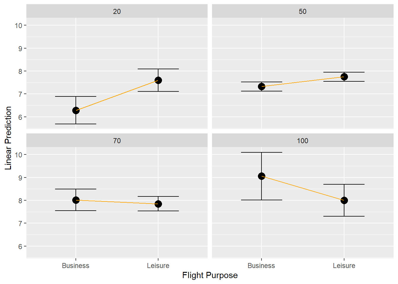
Figure 3.5: Margin plot (factor IV with continuous IV interaction)
Video Tutorial: lm() - Margin Plots for Factor IV with Continuous IV Interaction
3.4.6 Continuous IV (Interaction with Continuous IV)
# Run new model with 'age' and 'overall_sat' interaction
model4 <- lm(nps ~ age*overall_sat + nflights, airlinesat)
summary(model4)
Call:
lm(formula = nps ~ age * overall_sat + nflights, data = airlinesat)

Residuals:
    Min      1Q  Median      3Q     Max
-7.9218 -0.9129  0.4645  1.4897  5.7636

Coefficients:
                 Estimate Std. Error t value Pr(>|t|)
(Intercept)      7.181885   0.748391   9.596  < 2e-16 ***
age             -0.023019   0.014642  -1.572  0.11623
overall_sat     -0.051154   0.177249  -0.289  0.77294
nflights        -0.007328   0.003370  -2.175  0.02986 *
age:overall_sat  0.009427   0.003448   2.734  0.00636 **
---
Signif. codes:  0 '***' 0.001 '**' 0.01 '*' 0.05 '.' 0.1 ' ' 1

Residual standard error: 2.205 on 1060 degrees of freedom
Multiple R-squared:  0.1068,    Adjusted R-squared:  0.1035
F-statistic: 31.7 on 4 and 1060 DF, p-value: < 2.2e-16# Create data frame with values to be plotted
# By default, 5 evenly-spaced values for 'overall_sat' will be created, but for
# easier interpretation, set 'xlevels=4'
age.pred <- data.frame(predictorEffect("age", model4, xlevels=4))
# Create plot
age.pred %>%
ggplot(aes(x=age, y=fit,
color=factor(overall_sat), fill=factor(overall_sat))) + # color based on factor
geom_line(size=1) + # Draw predicted line
geom_ribbon(aes(ymin=lower, # Draws the confidence interval bands
ymax=upper),
alpha=0.2) + # Sets transparency level
labs(x="Age", y="Linear Prediciton", color="Overall Satisfaction", fill="Overall Satisfaction") +
theme(legend.position="bottom")
Figure 3.6: Margin plot (continuous IV with continuous IV interaction)
Video Tutorial: lm() - Margin Plots for Continuous IV with Continuous IV Interaction
3.5 Margin Plots (User-Defined Function)
3.5.1 Overview
- The
mympuser-defined function can produce a margin plot (and margin table) for a single variable or for a variable that has an interaction with another variable.- Requires the following packages:
ggplot2dplyrggeffectsinsight
- Requires the following packages:
- Usage:
mymp(model, focal, int=NULL)where:modelis a saved linear regression (lm) model or binary logistic regression (glm, family="binomial") model.focalis the name of the focal predictor variable. Must be in quotations.intis the name of the interaction predictor variable. Must be in quotations. Can be excluded if focal variable only wanted (or no interaction exists).
- Objects returned:
$ptableis the margin table used to produce the plot$plotis the margin plot
- Notes:
- The function will automatically determine the variable type (i.e., continuous or factor) and create the plot accordingly.
3.5.2 Examples
- Using
model3from above, which was the following model: \(nps=\alpha+\beta_0age+\beta_1flight\_purpuse+\beta_3age\times{flight\_purpose}+\beta_4nflights+\varepsilon\) - In this model,
ageandnflightsare continuous, andflight_purposeis a factor.
# Focal variable only
## Output will be both "$ptable" and "$plot"
mymp(model=model3, focal="nflights")
$plot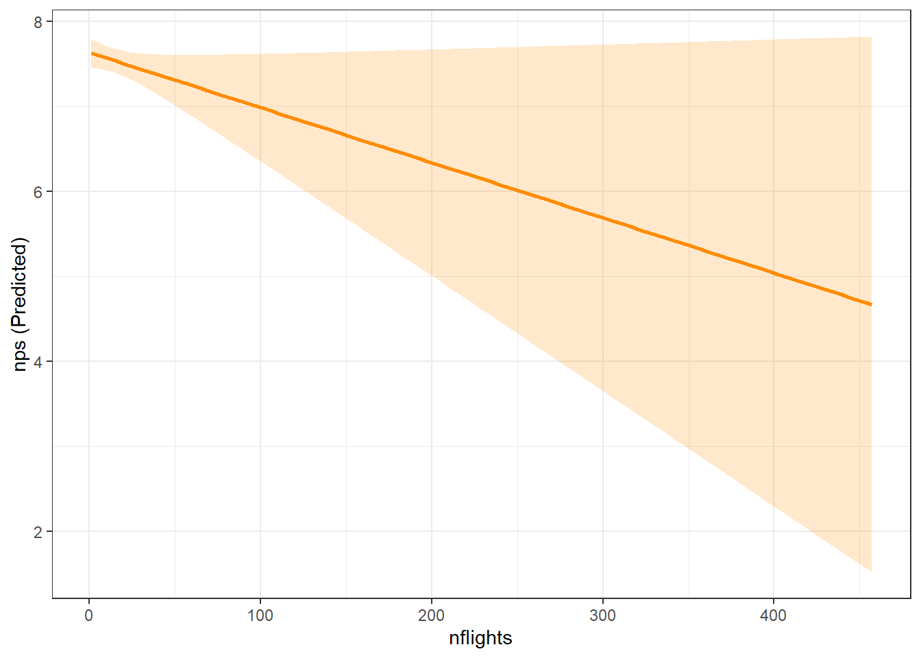
$ptable
# Predicted values of nps

nflights | Predicted |     95% CI
---------------------------------
       1 |      7.63 | 7.46, 7.79
      60 |      7.25 | 6.89, 7.61
     115 |      6.89 | 6.16, 7.62
     170 |      6.53 | 5.41, 7.65
     229 |      6.15 | 4.61, 7.69
     288 |      5.77 | 3.81, 7.72
     343 |      5.41 | 3.07, 7.75
     457 |      4.67 | 1.52, 7.82
# Focal variable and interaction
## Output will be "$plot" only
mymp(model3, "age", "flight_purpose")$plot