Chapter 12 Conjoint Analysis (Not Covered)

Data for this chapter:

The airlineca data is used from the MKT4320BGSU course package. Load the package and use the data() function to load the data.
```
# Load the course package
library(MKT4320BGSU)
# Load the data
data(airlineca)
```

12.1 Introduction

Base R does not have any built in function to handle conjoint analysis, because conjoint analysis can be done in a variety of ways. For this tutorial, the focus is on traditional conjoint using linear regression based methods. To accomplish the conjoint analysis, I have written a three user defined functions to help with getting the necessary results for traditional conjoint.

tradca produces overal part-worth plots for each attribute, and importance plot, and a table with case-level part-worths and importances
cademo produces correlation matrices and importance regressions from a dataframe of case-level part-worths/importances that has been appended with demographics
capred. compares two profiles specified by the user

12.2 `tradca` User Defined Function

Usage: tradca(formula, data, idvar="")
- formula is an object with a saved formula. The formula is represented by a DV on the left side separated from the IVs on the right side by a tilde(~). For traditional conjoint, the DV is the value rating for each profile, while the IVs are the name of the attribute variables. For example:
  - caform = value ~ attr1 + attr2 + attr3
- data is the name of the dataframe with the value ratings for each profile
- idvar is the variable that identifies the case (in quotes)
When saved to an object, this function will return three things:
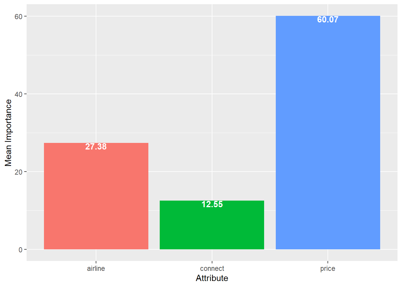
- pwplot contains a plot with average part-worth values for each attribute
- impplot contains a plot with the average importances
- casetable contains a dataframe with the part-worths and importances for each case
NOTE: This function requires the following packages:
- broom
- dplyr
- stringr
- ggplot2

# Load necessary packages
library(broom)
library(dplyr)
library(stringr)
library(ggplot2)

# Saving formula to object
caform <- value ~ airline + connect + price

# Using fucntion and saving to object called 'results'
results <- tradca(formula = caform,  # Formula object created above
                  data = airlineca,  # Data frame with profile ratings
                  idvar="caseid")    # Case id variable

results$pwplot   # Get part worth plot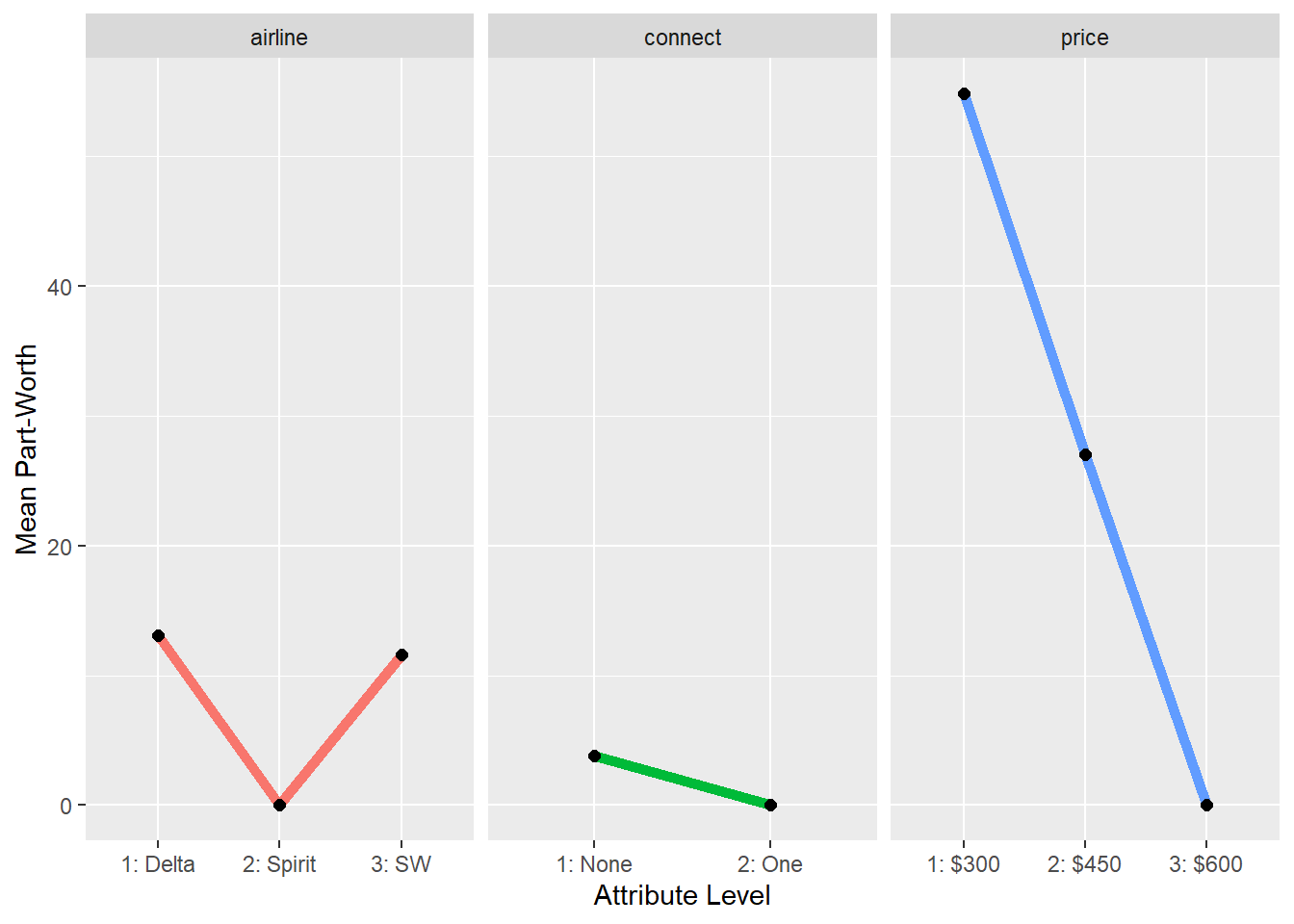

results$impplot  # Get importance plot

12.3 `cademo` User Defined Function

Usage: cademo(formula, data, vars="")
- formula is the saved formula object from before
- data is the name of the dataframe with case-level part-worths and importances, along with the appended demographic variables (see Preparation below)
- vars is a list of the demographic variable names
When run, this function will return correlation matrices and importance regressions depending on the type of demographic variable
NOTE: This function requires the Hmisc package

12.3.1 Preparation

To use this function, the casetable from the call to the tradca function must be appended with the demographic variables for each case. To do this, use the following code:

demos <- airlineca %>%   # Create new dataframe called 'demos' based on original data
   group_by(caseid) %>%      # Group by the 'idvar'
   summarise(inc=first(inc),    # Capture the demographic variables
             type=first(type)) %>% 
   bind_cols(.,results$casetable[,2:ncol(results$casetable)])  

# NOTE:  This last command appends the demographic variables 'casetable' dataframe

12.3.2 Function usage

cademo(caform,  # Formula object from before
       demos,   # Dataframe created above
       c("inc", "type"))  # Names of the demographic variables


Correlation Matrix for airline_
                     inc
airline_1: Delta   0.36*
airline_2: Spirit   0.17
airline_3: SW      0.36*

Correlation Matrix for connect_
                  inc
connect_1: None -0.01
connect_2: One   0.20

Correlation Matrix for price_
                 inc
price_1: $300 -0.35*
price_2: $450  -0.17
price_3: $600  -0.09

Correlation Matrix for Imp
               inc
Imp_airline  0.47*
Imp_connect   0.17
Imp_price   -0.48*

Regression Results for Imp_airline
             Estimate Std. Error t value Pr(>|t|)
(Intercept)   10.1131     7.5592  1.3379   0.1891
inc            0.3325     0.0946  3.5161   0.0012
typePleasure  -9.4936     5.3744 -1.7664   0.0856

Regression Results for Imp_connect
             Estimate Std. Error t value Pr(>|t|)
(Intercept)   10.2144     5.3877  1.8959   0.0658
inc            0.0787     0.0674  1.1672   0.2506
typePleasure  -5.0497     3.8305 -1.3183   0.1955

Regression Results for Imp_price
             Estimate Std. Error t value Pr(>|t|)
(Intercept)   79.6701     8.7485  9.1068   0.0000
inc           -0.4111     0.1094 -3.7567   0.0006
typePleasure  14.5439     6.2200  2.3382   0.0249

12.4 `capred` User Defined Function

Usage: cademo(formula, data, prof1, prof2)
- formula is the saved formula object from before
- data is the name of the dataframe with case-level part-worths and importances; this is the casetable object from the original call to the tradca function
- prof1 is the first profile (see Preparation below)
- prof2 is the second profile (see Preparation below)
When run, this function will return correlation matrices and importance regressions depending on the type of demographic variable

12.4.1 Preparation

To use this function, it works best to create the profiles by saving them to separate objects. The attribute levels for the profiles should be in the form of: attribute_levelnumber.
- For example, for the first Delta is the first level of the airline attribute, so we would use airline_1 to indicate that level of that attribute

# Create first profile
prof1 <- c("airline_1", "connect_2", "price_3")
# Create second profile
prof2 <- c("airline_3", "connect_2", "price_2")

12.4.2 Function usage

capred(caform,  # Formula object from before
       results$casetable,   # Dataframe from original 'tradca' call
       prof1, prof2)  # Names of our profile objects


Profile 1 = airline_1: Delta  /  connect_2: One  /  price_3: $600
Mean Utility = 26.382
95% CI = (18.107,34.657)

Profile 2 = airline_3: SW  /  connect_2: One  /  price_2: $450
Mean Utility = 51.933
95% CI = (42.208,61.658)