Chapter 13 Forecasting II (Not Covered)
Data for this chapter:
The
msalesandqalesdata are used from theMKT4320BGSUcourse package. Load the package and use thedata()function to load the data.
13.1 Introduction
While Base R does have some time-series forecasting capabilities, there are several packages that make working with the data and running the analysis easier. For our class, we will be mainly using the fpp3 package inside of some user-defined functions. The user-defined functions are described briefly below, and then in detail in their own sections.
13.1.1 User-Defined Functions for Forecasting II
acplotscreates ACF and PACF plots needed for ARIMA forecastingtswh.noisecreates a cumulative periodogram and white noise test needed for ARIMA forecastingautoarimaruns an ARIMA model as specified by the user and an automatic search for the “best” model if requestedtsplotproduces a time series plot of the data (covered in Forecasting I)fccomparecompares models from saved results after running the methods functions (covered in Forecasting I)
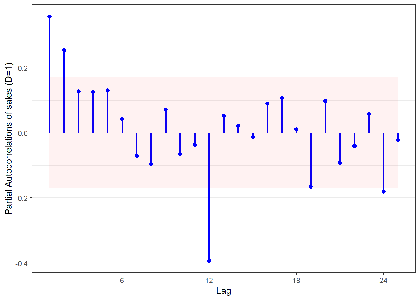
13.2 acplots User Defined Function
- Usage:
acplots(data, tvar="", obs="", datetype=c("ym", "yq", "yw"), h= , lags=, d=, D=c(0,1))datais the name of the dataframe with the time variable and measure variabletvaris the variable that identifies the time period (in quotes)obsis the variable that identifies the measure (in quotes)datetypecan be one of three options:"ym"if the time period is year-month"yq"if the time period is year-quarter"yw"if the time period is year-week
his an integer indicating the number of holdout/forecast periodslagsis an integer indicating how many lags should be shown on the plot; default is 25dis the order of non-seasonal differencing; default is 0Dis the order of seasonal differencing; default is 0
- NOTE: The results of this function can be saved to an object. When doing so, the following objects are returned:
$acfcontains the ACF plot$pacfcontains the PACF plot
out <- acplots(msales, "t", "sales", "ym", 12,
               lags=25,   # Number of lags to plot
               d=0,       # Non-seasonal differencing
               D=1)       # Seasonal differencing
out$acf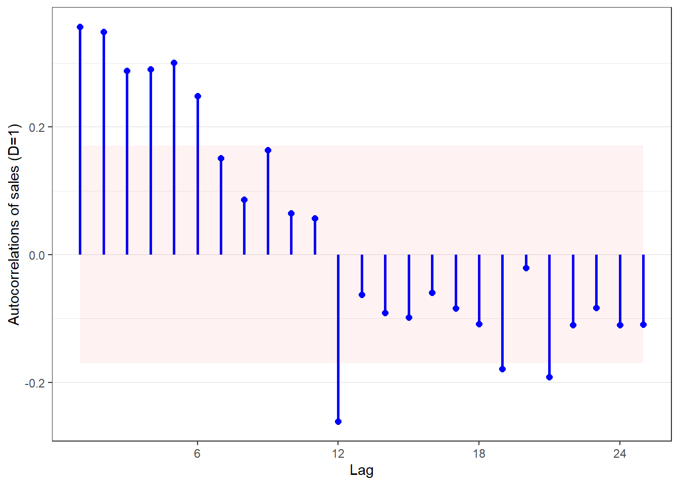
13.3 tswh.noise User Defined Function
- Usage:
tswh.noise(data, tvar="", obs="", datetype=c("ym", "yq", "yw"), h= , arima=c(p,d,q), sarima=c(P,D,Q))datais the name of the dataframe with the time variable and measure variabletvaris the variable that identifies the time period (in quotes)obsis the variable that identifies the measure (in quotes)datetypecan be one of three options:"ym"if the time period is year-month"yq"if the time period is year-quarter"yw"if the time period is year-week
his an integer indicating the number of holdout/forecast periodslagsis an integer indicating how many lags should be shown on the plot; default is 25arima=(p,d,q)provides the non-seasonal autoregressive (\(p\)), differencing (\(d\)), and moving average (\(q\)) parameters, in the form ofc(p,d,q)where the parameters are integerssarima=(P,D,Q)provides the seasonal autoregressive (\(P\)), differencing (\(D\)), and moving average (\(Q\)) parameters, in the form ofc(P,D,Q)where the parameters are integers
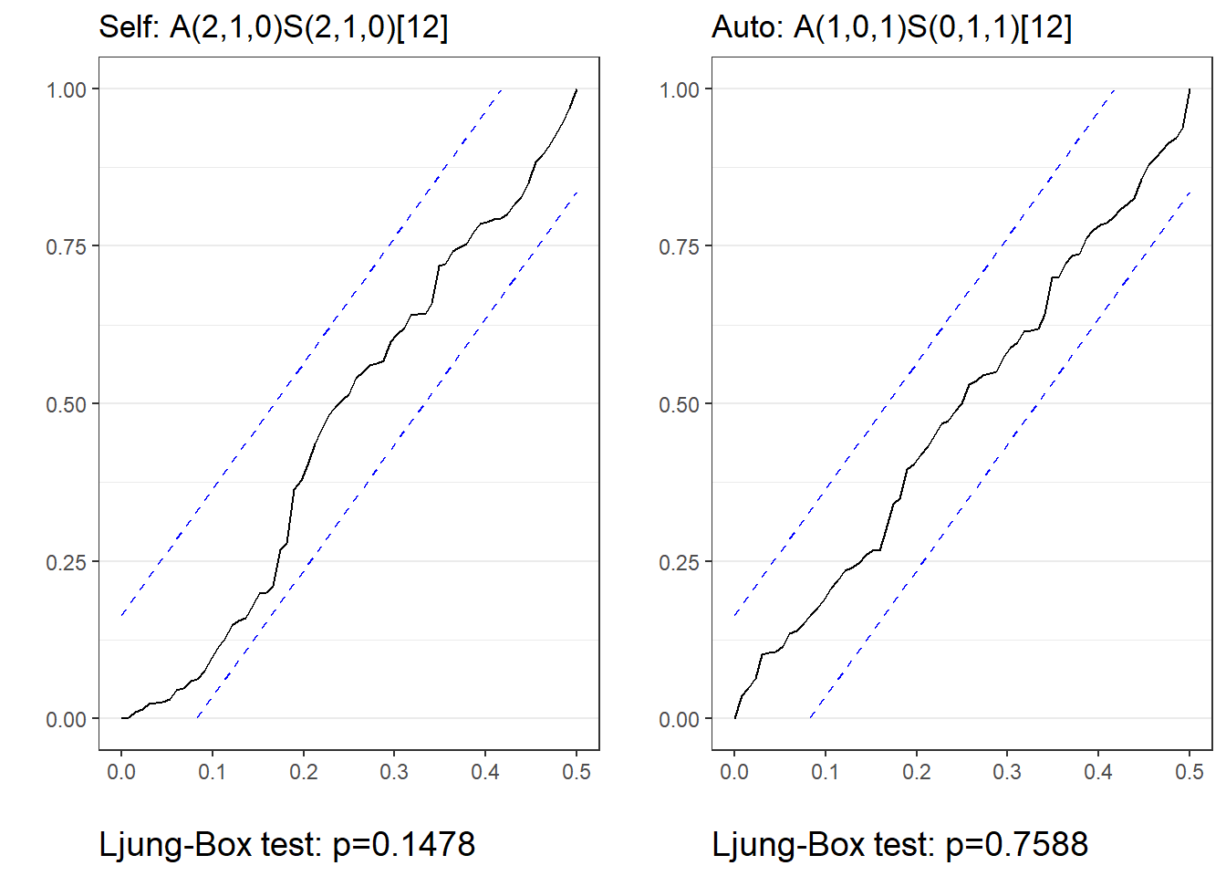
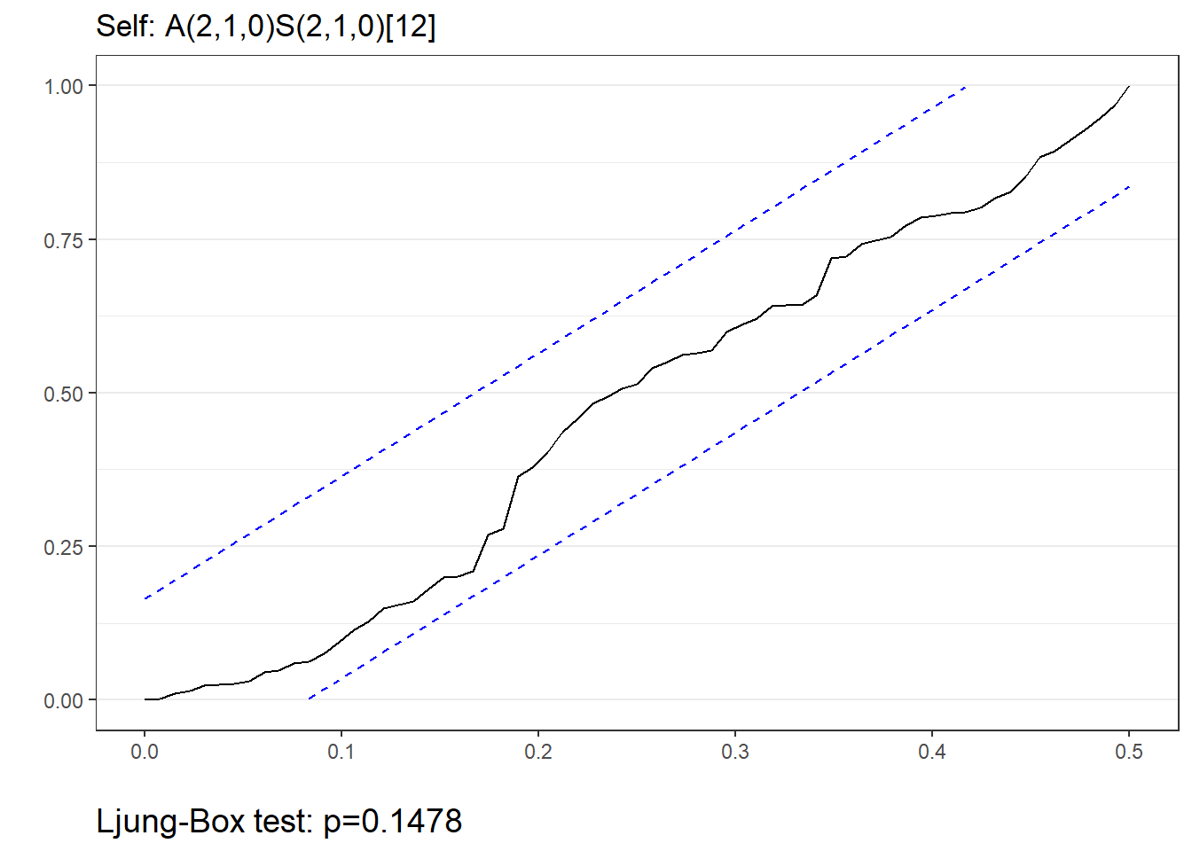
- The function will return a cumulative periodogram and results of the Ljung-Box White Noise test
tswh.noise(msales, "t", "sales", "ym", 12,
           arima=c(0,0,0),     # Seasonal parameters
           sarima=c(0,0,0))    # Non-seasonal parameters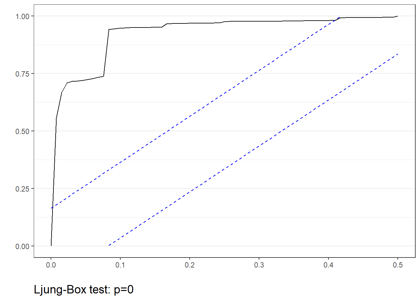
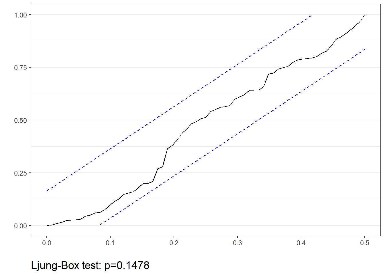
13.4 autoarima User Defined Function
- Usage:
tswh.noise(data, tvar="", obs="", datetype=c("ym", "yq", "yw"), h= , arima=c(p,d,q), sarima=c(P,D,Q), auto="")datais the name of the dataframe with the time variable and measure variabletvaris the variable that identifies the time period (in quotes)obsis the variable that identifies the measure (in quotes)datetypecan be one of three options:"ym"if the time period is year-month"yq"if the time period is year-quarter"yw"if the time period is year-week
his an integer indicating the number of holdout/forecast periodslagsis an integer indicating how many lags should be shown on the plot; default is 25arima=(p,d,q)provides the non-seasonal autoregressive (\(p\)), differencing (\(d\)), and moving average (\(q\)) parameters, in the form ofc(p,d,q)where the parameters are integerssarima=(P,D,Q)provides the seasonal autoregressive (\(P\)), differencing (\(D\)), and moving average (\(Q\)) parameters, in the form ofc(P,D,Q)where the parameters are integersautocan be one of two options:"Y"an automatic search is performed to find the “best” model"N"an automatic search is not performed
- NOTE 1: The results of this function should be saved to an object. When doing so, the following objects are returned:
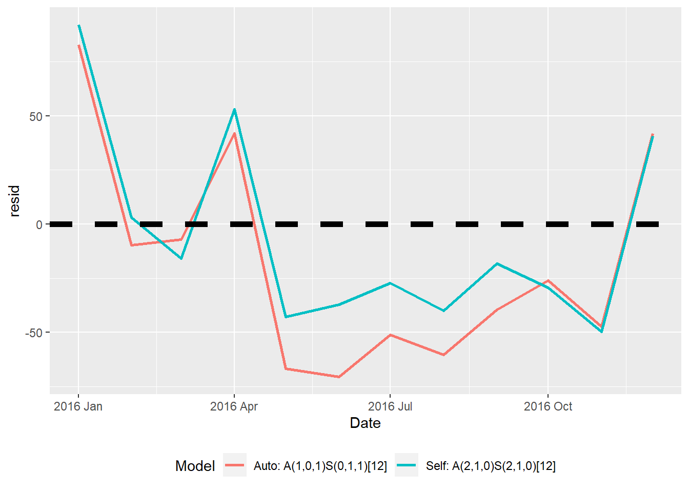
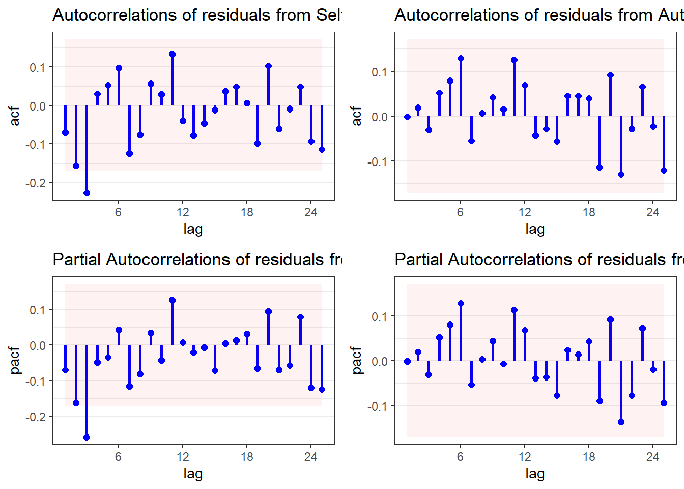
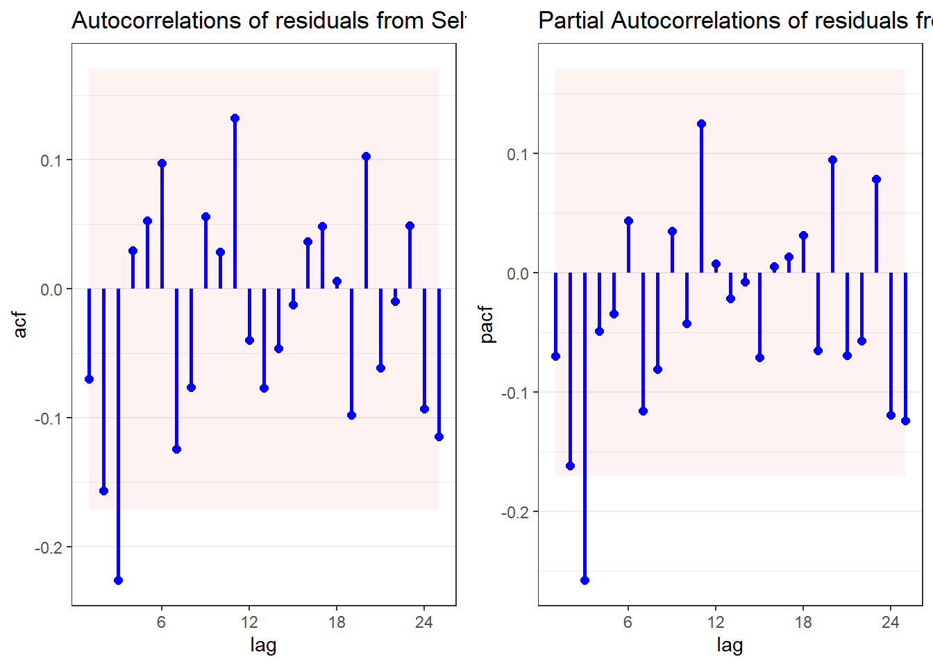
$plotcontains the ARIMA methods plot$acccontains the accuracy measures$fcresplotcontains a plot of the holdout period residuals$fcresidis a dataframe of the holdout period residuals (seldom used separately)$acresidcontains a plot of the ACF/PACF residuals for the model(s)$wncontains cumulative periodogram(s) and results of the Ljung-Box White Noise test(s)
- Note 2: If
auto="Y"is specified, this function can take one to two minutes to run - Note 3: The model names are:
- Self for the model specified by the user
- Auto for the “best” model if requested by the user
selfonly <- autoarima(msales, "t", "sales", "ym", 12,
                      arima=c(2,1,0),     # Seasonal parameters
                      sarima=c(2,1,0),    # Non-seasonal parameters
                      auto="N")           # Do not perform auto search
selfonly$plot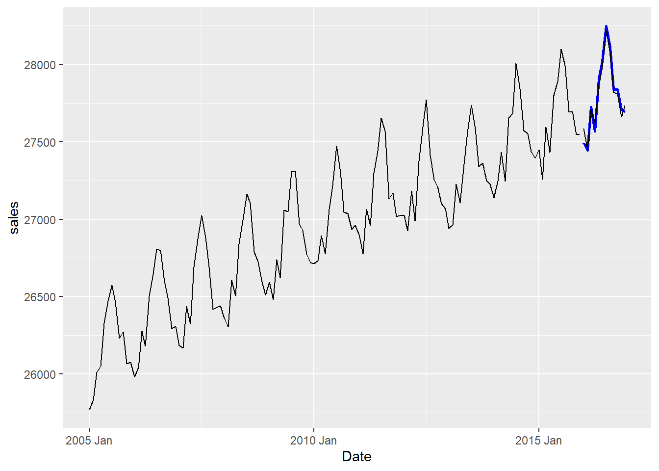
                       Model   RMSE    MAE  MAPE     AICc
1 Self: A(2,1,0)S(2,1,0)[12] 43.166 37.388 0.135 1359.636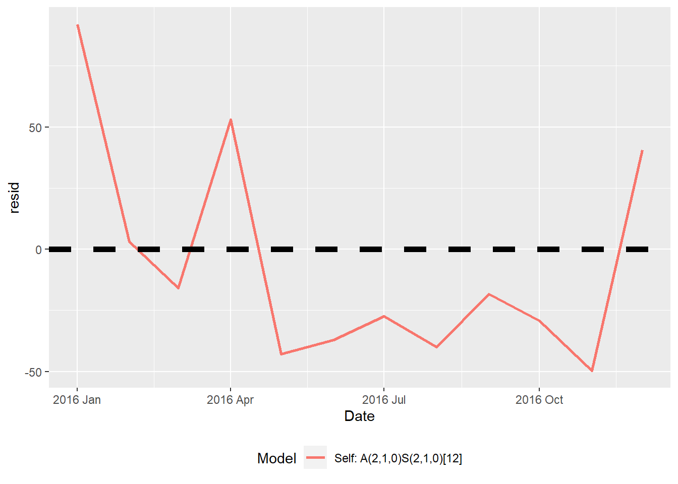
arima <- autoarima(msales, "t", "sales", "ym", 12,
                   arima=c(2,1,0),     # Seasonal parameters
                   sarima=c(2,1,0),    # Non-seasonal parameters
                   auto="Y")           # Do not perform auto search
arima$plot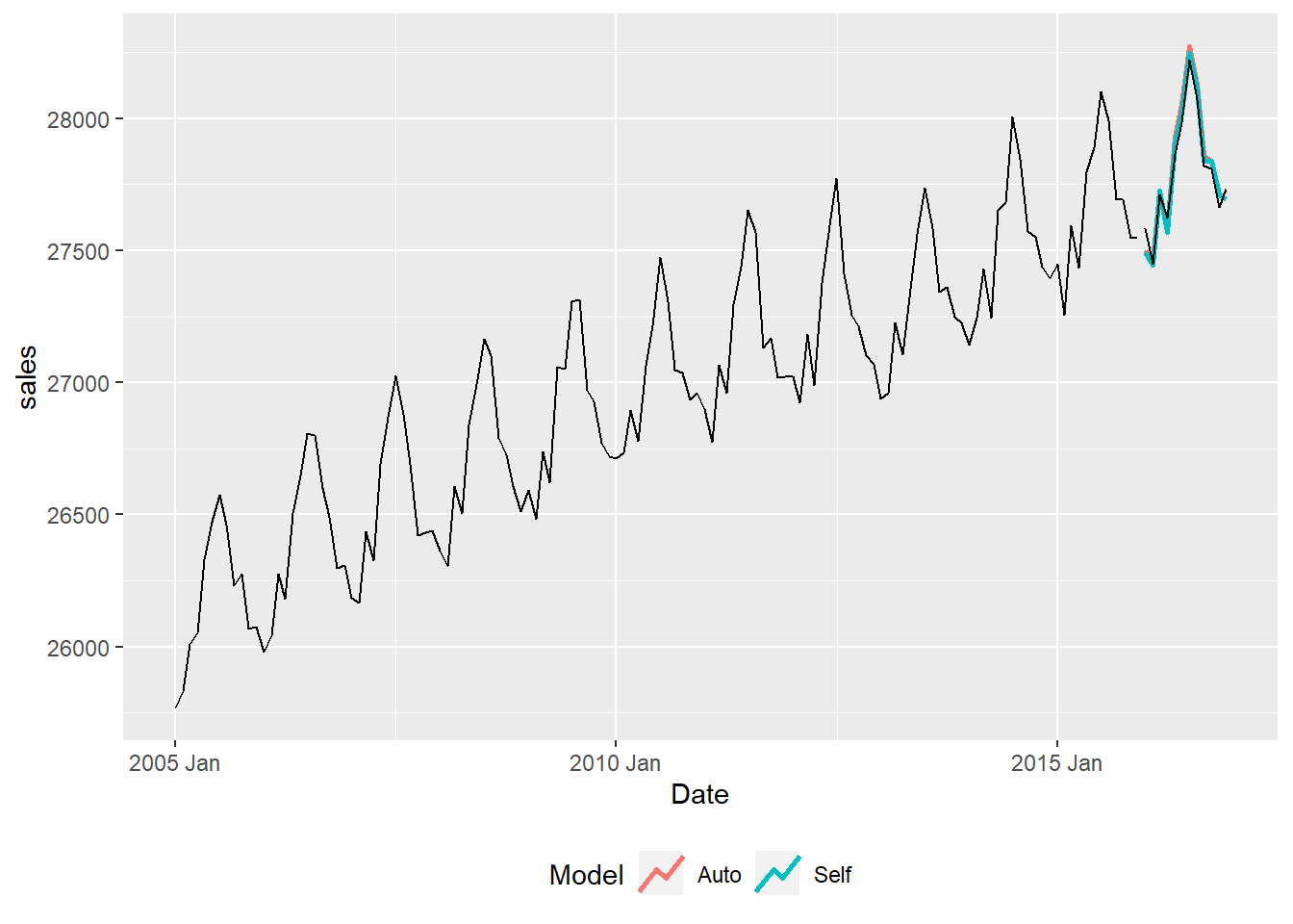
                       Model   RMSE    MAE  MAPE     AICc
1 Auto: A(1,0,1)S(0,1,1)[12] 50.531 45.393 0.163 1347.420
2 Self: A(2,1,0)S(2,1,0)[12] 43.166 37.388 0.135 1359.636